How AI Mastering Algorithms Work (Without the Math PhD)

Why Mastering Needed an AI Revolution

Mastering used to be the dark art reserved for golden‑eared engineers in multi‑million‑dollar rooms. Then came automated services like LANDR, eMastered, and modern advanced AI solutions such as our own Valkyrie AI Mastering by Beats To Rap On.

Curious how these neural tricks will evolve? AI Audio Mastering: What’s Next?

What changed?

1. CPU + GPU horsepower got cheap.
2. Deep‑learning breakthroughs (especially in image and speech domains) were ripe for cross‑pollination.
3. The MIR community produced 25 years of open research, culminating in the open‑access survey“ Twenty‑Five Years of Music Information Retrieval.”

Together these unlocked end‑to‑end models that can analyse a song in seconds, predict human‑style mastering moves, and spit out a loud, streaming‑ready WAV—no knobs required. The rest of this post unpacks the two pillars that make it possible:

1. Convolutional–Recurrent Neural Networks (CRNNs) – the pattern‑spotters that also remember context.
2. Spectral learning – the trick of turning noisy waveforms into “pictures of sound” a network can read.

---

1 · Convolutional–Recurrent Networks (CRNNs)

1.1 The 30‑second elevator pitch

1.3 Inside a typical CRNN mastering brain

Stage	Data shape	Role
Input	128 mel × 2,048 frames	Raw log‑mel spectrogram (~30 s chunk)
Conv 1	64 maps × 1,024 frames	Captures basic timbre edges
Conv 2	128 maps × 512 frames	Learns pitch‑harmonic blobs & percussive spikes
Conv 3	256 maps × 256 frames	Detects chords, rhythmic bursts, saturation fingerprints
Bi‑LSTM × 2	2 × 512 units	Reads forward & backward in time, modelling build‑ups & drops
Attention layer	256 units	Weighs the most influential moments (e.g., choruses)
Dense / heads	Multi‑task	One neuron bank predicts gain/EQ curves; another flags true‑peak risk; another tags emotion ↔ reference loudness

(Architectural numbers are illustrative but typical of systems documented in the ISMIR 2024 conference.)

1.4 Training a CRNN without losing your sanity

1. Curate massive audio corpora – commercial tracks, stems, and even lo‑fi bedroom demos. Diversity matters because networks will otherwise over‑fit to one style.
2. Generate teacher labels – either crowdsourced mastering moves, analytic DSP measurements (LUFS, crest factor, true‑peak), or expert‑engineer sessions exported as automation curves.
3. Augment aggressively – pitch‑shift, time‑stretch, stem‑swap drums, add noise. Each augmentation teaches the CNN to ignore irrelevant changes while preserving musical identity.
4. Multi‑task learning – predicting several targets at once (loudness, EQ, clarity) acts as a regulariser and encourages richer internal representations.
5. Progressive length scheduling – start with 5‑second clips (fast gradients), gradually feed 30‑second mixes so the RNN learns long‑form structure.

Want a hands‑on codebase? Check the GitHub repo for BeatNet; although aimed at beat tracking, its Torch data‑pipeline is 90 % transferable to mastering research.

1.5 Limitations & ongoing research

• Memory bottlenecks: LSTMs still struggle with tracks > 5 minutes. Researchers are experimenting with conformer and RWKV hybrids that marry self‑attention and recurrence.
• Explainability: A CRNN might recommend a 2 dB high‑shelf at 10 kHz—great, but why? Papers on saliency maps for audio (e.g., Grad‑CAM‑style overlays on spectrograms) aim to expose the decision logic.
• Latency: Real‑time mastering (live streaming) requires sub‑500 ms buffer windows. Lightweight GRU models paired with pruning / quantisation are hitting mobile‑chip targets in 2025 prototypes.

---

2 · Spectral Learning—Seeing Sound as an Image

2.1 From air pressure to heat‑map

Raw audio is simply amplitude over time. Our ears decode it, but neural nets choke on the sheer sample rate (44,100 floating‑points per second). Spectral learning flips the problem into two dimensions:

1. Slice the waveform into overlapping windows (20–50 ms)
2. Transform each slice with an FFT
3. Map those linear frequencies onto the Mel scale so bins align with how we perceive pitch
4. Log‑compress the magnitudes to imitate loudness perception

The result is a log‑mel spectrogram—an image whose colour intensity shows energy at each pitch band over time.

2.2 Spectrogram flavours your DSP‑chef should know

Name	Key trait	When it shines
Mel‑spectrogram	Perceptually spaced bins	General MIR & mastering
Constant‑Q	Log‑frequency basis (musical cents)	Chord/key analysis
CQT‑VQT hybrid	Variable Q across octaves	Transcription & poly‑instrument mixes
Chromagram	12 pitch‑class roll‑ups	Modulation tracking
ERB‑scale spec	Human cochlear spacing	Psychoacoustic masking research

2.3 Handy spectral descriptors (the “old‑school” features)

Even if deep models learn everything implicitly, classic descriptors still add transparency:

• Spectral centroid – average brightness; EDM drops often spike here, jazz brushes sit lower.
• Spectral flatness – noisiness vs tonality; white noise = 1, pure sine = 0.
• Zero‑crossing rate – quick’n’dirty way to gauge distortion or hiss.
• Spectral decay – slope after percussive attack; reveals reverb tails or tape saturation.
• MFCCs – 13‑vector snapshot of the spectral envelope; killer for instrument ID, less so for mastering because they ignore per‑bin loudness peaks.

Modern mastering AIs sometimes concatenate these “symbolic” vectors with CNN embeddings, giving the decision head a mix of explicit and learned insight.

---

3 · The AI Mastering Pipeline—End‑to‑End Walkthrough

Below is a representative flow adapted from our in‑house Valkyrie stack and open papers like Self‑Supervised Perceptual Loudness Prediction.

3.1 Stage A: Pre‑flight checks

1. Sample‑rate validation (resample if needed)
2. True‑peak scan using 4× oversampling to avoid inter‑sample overshoot
3. Phase correlation test for mono compatibility
4. LUFS anchor – initial integrated loudness reading sets baseline gain compensation

3.2 Stage B: Feature extraction & neural analysis

• Log‑mel spectrogram computed at 48 kHz → 512‑hop → 128 bins
• Spectral descriptor cache (centroid, roll‑off, crest factor)
• Stem estimation (optional) via Demucs to separate vocals vs drums, giving the CRNN stem‑aware channels to focus on

3.3 Stage C: CRNN inference

The “brain” we dissected earlier. Outputs include:

Head	Prediction	Use‑case
Dynamic EQ curve	24‑band gain values	Automated tonal shaping
Compressor map	Threshold & ratio per band	Multiband dynamics
Stereo image target	Mid/side spread suggestions	Width enhancement
Limiter ceiling	dBTP value	Streaming compliance
Genre / mood tag	One‑hot vectors	Genre‑aware preset interpolation

3.4 Stage D: DSP rendering engine

A deterministic signal‑processing chain applies the neural recommendations:

1. Static pre‑EQ – gentle shelf corrections the model marked as “always‑on.”
2. Multiband compression driven by the CRNN map with look‑ahead to preserve transients.
3. Dynamic EQ (e.g., Weiss EQ MP) modulated by side‑chain triggers (harsh S’s, boomy toms).
4. Harmonic exciter / tape saturator engaged conditionally when spectral flatness dips below a learned threshold (indicating dullness).
5. Stereo enhancer – MS matrix widener with correlation guardrails.
6. True‑peak limiter – oversampled (8×) brick‑wall, ceiling according to predicted headroom.
7. Metering & loudness match – auto‑level post‑processing to within ±0.1 LU of the CRNN’s target.

3.5 Stage E: Validation & user preview

• Before/After loudness match to avoid the “louder is better” psychoacoustic bias.
• Spectrogram diff view in the UI overlays hot‑spots, letting users see what the AI tweaked.
• Interactive tweak layer: Producers can nudge “Warmth,” “Punch,” or “Air” sliders that translate to simple offsets in the CRNN’s parameter space—so the AI remains in the loop.

---

4 · Case Study: From Bedroom Demo to Streaming‑Ready in 60 Seconds

Track: “Late‑Night Bounce” – 2‑minute lo‑fi beat at 74 BPM, heavy side‑chain kick, murky Rhodes chords.

1. Ingest – 16‑bit/44.1 kHz WAV; AI detects −18 LUFS integrated, 0 dBTP peaks (danger).
2. Analysis – CRNN tags genre as “Lo‑Fi Hip‑Hop,” mood “Chill,” tempo 74 BPM.
3. Moves it made:
   • High‑pass EQ at 25 Hz to clear sub‑rumble.
   • Dynamic EQ ducks 500 Hz whenever kick hits—reduces mud.
   • Tape saturation module engaged at 3 % THD for cozy warmth.
   • Stereo widener adds subtle side energy above 3 kHz.
   • Limiter set to −1 dBTP, final loudness −14 LUFS (Spotify safe).
4. Output – WAV 24‑bit/48 kHz + MP3 320 kbps.
5. Time elapsed: 43 seconds on a MacBook M2.

Listening back, the kick sits cleanly, Rhodes shimmer without harshness, overall loudness matches the Spotify loudness guideline, and no clip lights on the true‑peak meter.

---

5 · Frequently Asked Questions

Q 1: Does AI mastering replace human engineers?

Not for critical albums needing bespoke artistry. But for singles, demos, podcasts, or creators on a budget, AI offers 80 % of the polish in a fraction of the time.

Q 2: Why not analyse the raw waveform directly?

Raw PCM at 44,100 Hz is too verbose. Spectral transforms compress the data, align with psychoacoustics, and present the CNN with image‑like structures it evolved to decode.

Q 3: Can I trick the CRNN by inserting pink noise or weird instruments?

You can confuse it—researchers already found adversarial examples—but production‑grade systems add jitter, augmentation, and sanity‑checks (phase coherence, crest factor bounds) to stay robust.

Q 4: What about Dolby Atmos / multichannel?

Multi‑stem workflows feed each bed or object to separate CRNN branches, then fuse predictions via attention layers. Expect fully automated Atmos mastering by 2026.

---

6 · Peering Into the Future

1. Self‑supervised pre‑training – Models learn from millions of unlabeled tracks using contrastive audio tasks, then fine‑tune on small expert data.
2. Diffusion‑based resynthesis – Imagine a mastering engine that “redraws” the mix’s spectrogram with target tonal balance, rather than merely EQing the original. Early labs report fewer artifacts.
3. Real‑time feedback loops – Latency‑optimised CRNNs inside DAWs, adjusting compressor thresholds on the fly as you tweak faders.
4. Explainable AI dashboards – Saliency overlays on spectrograms so you see exactly which drum transient triggered that 1 dB gain reduction.
5. Edge deployment – ARM‑optimised inference lets a phone master live concert footage before it even hits Instagram Stories.

---

7 · Take‑Home Nuggets

• Spectral learning turns sound into a colourful canvas; CRNNs bring painterly vision plus temporal memory.
• The pairing powers not just mastering, but beat tracking, key detection, mood tagging, even automatic stem remixing.
• Robust AI mastering stacks aren’t magic black boxes—they’re deterministic DSP chains guided by neural predictions, audited by loudness and true‑peak meters.

So next time you upload a track to an “instant‑master” platform, picture a heat‑map flickering under convolutional microscopes, with an RNN tapping along to your groove. That’s the brain deciding whether your low‑end needs trimming or your hi‑hats deserve extra sparkle—and it all happens before you can top up your coffee.

---

Further Exploration (all clickable)

Twenty‑Five Years of MIR Research – landmark survey, 400+ references. BeatNet – state‑of‑the‑art CRNN for beat + downbeat tracking. Audio Feature Extraction – practical walkthrough of mel‑spectrograms and MFCCs. Demucs – neural stem‑separator that underpins many mixing/mastering workflows. Spotify Loudness Normalisation – know your LUFS targets.

Music Information Retrieval (MIR) is a field devoted to analyzing, understanding, and organizing music through computational methods. Two fundamental approaches in modern MIR are convolutional–recurrent neural networks (CRNNs) and spectral learning techniques. In simple terms, CRNNs combine convolutional neural networks (CNNs) (good at extracting patterns from images or spectrograms) with recurrent neural networks (RNNs) (good at handling sequences) to model musical audio. Spectral learning refers to analyzing audio in the frequency domain (using representations like spectrograms) to extract meaningful features about the sound. This article breaks down these concepts in intuitive terms, explaining how they work and how they are applied in MIR tasks like genre recognition, beat tracking, and emotion detection. We’ll use insights (and diagrams) from a comprehensive 2024 MIR survey as our guide, keeping the explanations accessible and focusing on core ideas rather than complex math.

Convolutional–Recurrent Networks (CRNNs) in Music Analysis

What is a CRNN? A convolutional–recurrent network is essentially a hybrid of two neural network types: a CNN followed by an RNN medium.commedium.com. In an audio context, we typically first convert the sound into an image-like representation (a spectrogram, explained later) and feed that into the CNN. The convolutional layers act like pattern detectors sliding over this time–frequency image, picking out local features such as specific note harmonics or drum attack patterns, regardless of where they occur in time dcase.community. The output of the CNN is a sequence of feature vectors (one per time slice, containing the detected pattern activations). Then the recurrent layers (e.g. an LSTM or GRU network) process this sequence in order, learning the temporal dependencies – in other words, how the music’s content unfolds over time dcase.community. The RNN has a memory, allowing it to integrate information across frames, which is crucial for music since musical meaning often lies in patterns across time (melodies, rhythms, progression of chords, etc.). Finally, a dense layer can map the RNN’s output to the desired prediction (such as a genre label or the timing of a beat).

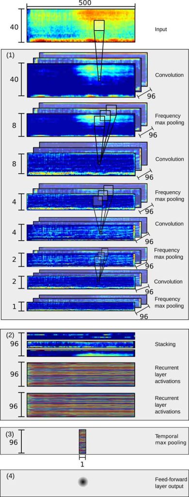
Figure: Example architecture of a convolutional–recurrent neural network for audio. The audio waveform is first converted into a time–frequency spectrogram image. Three convolutional layers (Conv1–Conv3) extract local spectral patterns at different levels, which are then fed into a bidirectional LSTM (recurrent layer) that captures temporal context. A final fully-connected layer (FC) produces the output (e.g. class probabilities for a classification task) researchgate.net. This combination allows the network to learn what sound patterns occur and when they occur.

In essence, CNNs handle the spatial structure of audio data (the frequency content within short time windows), and RNNs handle the temporal structure (the sequence of those short windows) dcase.community dcase.community. CNNs are good at recognizing local features like a chord’s frequency spectrum or a drum hit’s spike, independent of their position in time dcase.community. RNNs are good at remembering context, such as a recurring rhythm or melody motif, by maintaining a state or memory of what came before. By combining them, CRNNs can learn complex spectro-temporal patterns – for example, a certain riff (pattern in frequency) that repeats every few beats (pattern in time).

Key Points of CRNNs in MIR (Bullet Summary)

• Convolutional layers = feature extractors: They scan the spectrogram and detect local patterns (e.g. a particular instrument’s timbre or an onset) regardless of when they occur This is analogous to how image CNNs detect edges or shapes in pictures.
• Recurrent layers = sequence modelers: They take the sequence of features from the CNN and learn long-term dependencies. This enables modeling musical phrases, rhythms, or chord progressions over time.
• End-to-end learning: CRNNs can be trained directly on audio data transformed into spectrograms, learning features automatically instead of relying on hand-crafted rules. This often yields better performance in practice, since the network can optimize features for the specific task.

Applications of CRNNs in MIR

CRNN architectures have been successfully applied to various MIR tasks that have both spectral and temporal complexity:

• Music Genre Recognition: Music genre classification benefits from CRNNs by capturing both the timbral characteristics of genres and their temporal patterns. For instance, a CNN can identify instrumentation or texture (e.g. distorted guitar vs. strings), while an RNN can capture rhythmic or structural patterns (like the presence of a drop in EDM or a verse-chorus cycle in pop). Research has shown that using CNNs or CRNNs on spectrogram inputs yields strong performance in music classification tasks arxiv.org. The CNN part might detect, say, the spectral signature of a guitar riff or a vocal melisma, and the RNN part can learn that certain sequences of these signatures are characteristic of rock versus R&B (for example). In the 2024 MIR survey, it’s noted that deep networks (CNNs and CRNNs) now outperform earlier approaches that used hand-crafted audio features for classification.
• Beat Tracking and Rhythm Analysis: Detecting the beat of a song is a temporal task that also relies on spectral cues (drum hits are broadband sounds). CRNNs have proven effective here by identifying short-term percussive events and then linking them over time. A prime example is BeatNet, a model that uses a convolutional front-end to detect onset patterns and a recurrent back-end (plus a filtering method) to track beats and downbeats continuously. The CNN picks up where in the spectrogram sharp, vertical lines occur (signatures of drum hits) and the RNN helps predict when the next hit is likely, given the learned tempo and meter. This combination allows real-time beat tracking with high accuracy, as reported in the literature arxiv.org.
• Emotion/Mood Detection: Music emotion recognition (MER) attempts to classify music by the feeling it evokes (happy, sad, energetic, etc.). This is a high-level task akin to genre tagging, and CRNNs are well-suited because emotional cues in music come from timbral qualities and how they change over time. A CRNN can learn, for example, that a “happy” song often has bright instrumentation and an upbeat rhythm, maintained throughout the track, whereas a “sad” piece might have mellower tones and slower, gradual developments. In MIR, mood recognition is treated as a clip-level classification problem similar to genre tagging. Therefore, architectures that work for genre (like CNNs or CRNNs on spectrograms) have also been applied to emotion detection. The CNN might capture brightness or the presence of certain instruments (like a heavy electric guitar might correlate with aggressive/angry moods), while the RNN could capture temporal dynamics (a slow evolution and minimal percussion might correlate with calmer emotions). By preserving temporal context, CRNNs can outperform models that look at only averaged features, especially for music where the emotional content builds or changes over time.

In summary, convolutional–recurrent networks provide a powerful, biologically inspired way to analyze music: they mimic how we might first notice instant sound qualities (timbre, notes) and then listen for patterns over time (rhythm, melody). This synergy is why the 2024 survey highlights CRNN variants in many state-of-the-art MIR systems.

Spectral Learning: Frequency-Domain Features in MIR

When we talk about spectral learning, we mean analyzing the frequency content of audio signals – essentially, breaking sound into its constituent frequencies (pitches) over time, and using those representations for learning. Music signals are naturally understood in the frequency domain: when we hear a chord, we perceive multiple frequencies at once; when we sense timbre, we’re noticing the spectral shape of the sound. Therefore, a core step in MIR is to transform audio from the raw waveform (amplitude vs time) into a spectrogram, which is a time–frequency representation. This transformation is typically done via the Short-Time Fourier Transform (STFT): the audio is chopped into short frames (e.g. ~20–50 ms), and each frame undergoes a Fourier transform to identify the frequencies present. Stacking these analyses over time yields a spectrogram – basically an image where the x-axis is time, the y-axis is frequency, and the intensity (color) indicates how strong each frequency is at each moment.

Notably, the 2024 MIR survey emphasizes that working in the frequency domain is advantageous for audio analysis: it reduces the data complexity while preserving important information about musical content. Direct waveform data is high-dimensional and harder for models to interpret, whereas a spectrogram highlights the meaningful structure (like harmonics, beats, etc.) in a more compact form. Often, a Mel-scale spectrogram is used – this is a spectrogram that has been scaled according to human pitch perception (frequencies are spaced more coarsely at high end and finely at low end, mimicking our ears) and usually converted to a logarithmic amplitude scale (dB). Using a Mel spectrogram further reduces dimensionality and focuses the representation on perceptually relevant aspects of sound dcase.community. In fact, many state-of-the-art MIR systems and deep models take mel-spectrograms as input because they strike a good balance between detail and manageability, and models trained on frequency-domain inputs often outperform those on raw waveforms.

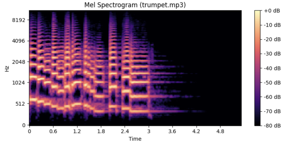
Figure: A mel-frequency spectrogram of an example audio signal (here, a spoken utterance is shown for illustration). Time progresses left-to-right, frequency (pitch) is on the vertical axis (low bass frequencies at bottom, high treble at top), and color intensity indicates the amplitude of each frequency at each moment. Clear patterns emerge in this spectrogram (for instance, horizontal striations from vocal harmonics and vertical spikes from certain consonant sounds), which makes the spectral representation a rich source of features for learning developer.nvidia.com. In music, a mel-spectrogram of a song would show, for example, sustained horizontal lines for steady notes, broadband bursts for drum hits, etc., all of which a model can learn to interpret.

How spectral features are extracted: In summary form, converting to the spectral domain involves a few steps:

• Fourier Transform: Convert the time-domain signal into frequencies (using FFT). For a changing signal like music, apply FFT on short overlapping frames via STFT arxiv.org.
• Mel Scaling: Apply a bank of filters that group the raw frequency bins into perceptual “pitch bands” (mel bands). The filter bandwidths increase with frequency, reflecting how our hearing has lower resolution at high frequencies arxiv.orgarxiv.org. This yields the Mel spectrogram.
• Log Compression: Convert magnitudes to a logarithmic scale (dB), which compresses the huge dynamic range of audio and aligns with human loudness perception arxiv.org. Now the spectrogram highlights perceptually significant changes in energy arxiv.org.
• (Optional) Feature Summary: Sometimes further transforms like the Discrete Cosine Transform are applied to the log-mel spectrogram to derive Mel-Frequency Cepstral Coefficients (MFCCs) – which compactly describe the spectral envelope (overall shape) of each frame arxiv.org. MFCCs have been widely used in MIR (borrowed from speech recognition) as a set of ~13 numbers per frame capturing timbral characteristics.

The end result is a set of features that tell us about the musical signal’s content in a frequency-centric way. For example, we can see which frequencies carry the most energy at a given time (is there a dominant pitch? lots of bass? presence of high-frequency percussion?), and how that pattern changes over the course of the track.

Why spectral learning matters for MIR

Most musical attributes are inherently spectral. Melodies and harmonies are about specific frequencies (notes) being present. Instrumentation and timbre are about the shape of the frequency spectrum. Rhythms often manifest as patterns of broadband energy bursts (percussive hits have energy across many frequencies at the onset). By analyzing these in the spectrogram, algorithms can detect musically meaningful events. The 2024 survey underscores that using frequency-domain representations generally improves the performance of learning algorithms on audio – indeed, “frequency domain is usually preferred” when training deep models on audio and many recent MIR advances have come from better spectral feature processing.

Key Points of Spectral Learning (Bullet Summary)

• Spectrogram = foundation: Converting audio to a spectrogram (especially mel-scaled, log-amplitude) is a foundational step. It reveals the structure of the music in time–frequency space, making it easier for models to learn patterns.
• Dimensionality reduction: Spectral methods like mel scaling and MFCCs greatly reduce data size while keeping important information. This simplifies learning (less “curse of dimensionality”) and emphasizes perceptually important features.
• Human-aligned features: The use of mel scale and log amplitude means the features align with how humans hear (pitch spacing and loudness), which often leads to more musically relevant analysis.
• Various spectral features: Aside from the raw spectrogram, MIR also uses derived spectral features – e.g. spectral centroid (the “brightness” of the sound, the center of mass of the spectrum) which correlates with timbre brightness medium.com, spectral roll-off (frequency below which most energy lies, indicating bandwidth), chroma features (which collapse the spectrum into 12 pitch classes to focus on harmony) useful for chord and key detection, and others. These can be used in combination or fed into machine learning models.

Applications of Spectral Learning in MIR

Virtually all MIR tasks involve spectral learning at some stage. Here’s how frequency-domain analysis contributes to our example tasks:

• Genre Recognition: Different music genres often have distinct spectral “signatures.” For instance, metal might have a wide spectrum with strong energy in guitar mid-frequencies and cymbal highs, while classical music might show clear harmonic lines from strings and less emphasis on extreme highs or lows. By using features like MFCCs, spectral centroid, or directly learning on spectrograms, classifiers can pick up on these distinctions. In a genre classification study, researchers improved accuracy by including features such as spectral roll-off, spectral centroid, and MFCCs, which capture timbral and spectral characteristics of the audio arxiv.org. Essentially, spectral features tell the model about the instrumentation and audio texture of the piece – crucial factors for genre. A spectrogram-based CNN (as part of a CRNN or alone) can automatically learn these genre-specific spectral patterns arxiv.org.
• Beat Tracking / Onset Detection: Beats are marked by sudden increases in energy across a broad range of frequencies (e.g. a drum hit has a noisy, wide-frequency spectrum). In the spectrogram, these show up as vertical streaks (energy spike at a moment across many frequencies). Spectral methods excel at detecting such changes: a common handcrafted feature is spectral flux, which measures the frame-to-frame change in the spectrum (large flux often indicates an onset). Modern deep learning methods likewise use spectrograms to find patterns of percussive events. As an illustrative point, if we separate a spectrogram into harmonic parts (horizontal lines) and percussive parts (vertical lines), the percussive component clearly highlights the beats medium.com. In MIR, algorithms use this property by either explicitly separating components or by letting a CNN learn to detect vertical patterns corresponding to drum hits. Once those onsets are detected (via spectral cues), higher-level processing can space them out to determine tempo. The spectral domain is indispensable here because a simple waveform doesn’t reveal these frequency-localized bursts as clearly as a spectrogram does. In summary, spectral learning techniques provide the when and what frequency content of events needed to identify beats and rhythmic structure.
• Emotion Detection: Emotions in music are often conveyed through instrumentation (timbre) and production (e.g. bright versus dark sound, heavy bass or not, etc.) as well as through musical elements like mode or tempo. Spectral features contribute significantly to quantifying these aspects. For example, an “aggressive” or energetic emotion might correlate with a broader, flatter spectrum (lots of high-frequency content, distorted guitar noise, etc.), whereas a “sad” or calm piece might have a mellower spectrum (energy concentrated in lower frequencies, smoother harmonic lines). The spectral centroid feature, which indicates whether the spectrum’s energy is more high-pitched or low-pitched on average, can serve as a proxy for brightness and has been used in mood recognition (brighter sounds often feel more energetic or happy) medium.com. Additionally, chroma features (which focus on pitches/chords) can help detect if a song is in a major key (often associated with happy emotions) or minor key (often sad), though emotion detection is more complex than just major/minor. In practice, models for music emotion classification input spectrogram-based representations into CNNs or CRNNs, just like genre models, because emotion recognition is treated similarly to a tagging task arxiv.org. Thus, they inherently leverage spectral learning. The 2024 survey lists mood/emotion recognition alongside genre recognition as “clip-level classification tasks” addressed by similar techniques arxiv.org. By examining spectral patterns (timbre, brightness, harmonic content) over time, these models learn to predict the emotional tag of a piece. For a concrete example, a network might learn that songs labeled “angry” have strong high-frequency content and rhythmic spectral bursts (driving percussion), whereas “sad” songs might exhibit softer high-end presence and slower, more sustained harmonic content.

In all these cases, the frequency-domain view is fundamental. It’s much like analyzing the light spectrum to understand the properties of a star in astrophysics – here we analyze the sound spectrum to understand properties of music. Spectral learning techniques give MIR systems a window into the structure of sound that aligns with musical concepts (pitch, harmony, timbre, rhythm), making them indispensable. As the survey highlights, combining spectral representations with advanced models (like CRNNs) has driven a lot of progress in MIR, enabling tasks like genre or mood classification, beat tracking, and many others to reach high accuracy by leveraging the rich information hidden in the frequency domain.

Conclusion

To summarize, convolutional–recurrent networks and spectral learning are complementary approaches that together form the backbone of many modern MIR systems. CRNNs provide a powerful architecture to learn both local audio features and their temporal relationships – much as our ears and brain together first parse instantaneous sound qualities and then integrate them over time. Spectral learning provides the appropriate “lens” for the data, transforming audio into a domain where musically relevant patterns are visible and learnable. An MIR system that identifies a song’s genre, taps along to its beat, or infers its emotional mood likely uses a spectrogram as input (thanks to spectral analysis) and a deep network with convolutional and possibly recurrent layers to make sense of it. By emphasizing intuitive patterns – like the shape of a sound in frequency space or the repetition of a motif over time – these methods allow even those without a Ph.D. in math to grasp the essence: we look at music as a picture of sound (spectrogram) and use smart pattern-recognizing modules (CNNs, RNNs) to understand that picture. This combination, as documented in the 2024 MIR survey, has proven remarkably effective across a wide range of tasks, bringing us closer to automated understanding of music in ways that often parallel our own human listening experience.

References

• Meinard Müller et al., “25 Years of Music Information Retrieval: 2024 Survey” (selected content on convolutional–recurrent networks and spectral audio features) dcase.community dcase.community arxiv.org arxiv.org.
• Anuradha Chopra et al., “MIRFLEX: Music Information Retrieval Feature Library for Extraction” (ISMIR 2024 extended abstract) – tables of MIR methods, including BeatNet CRNN for beat tracking arxiv.org.
• Friedrich Wolf-Monheim, “Spectral and Rhythm Features for Audio Classification with Deep CNNs” (arXiv 2024) – examples of spectrograms and spectral features medium.com arxiv.org.
• Chao Sun et al., “CRNN-A for Speech Separation” (Scientific Reports 2021) – description of CNN front-end + RNN back-end for audio, highlighting translation-invariant feature extraction and sequence modeling nature.com. (Concept applies similarly to music signals.)
• Katsiaryna Ruksha, “Music Information Retrieval: Feature Engineering” (Medium, 2021) – intuitive tutorial on audio features (mel spectrogram, MFCC, chroma, etc.) with genre examples medium.com. (Provides accessible explanations of spectral features relevant to MIR.)