Demucs vs Spleeter – The Ultimate Guide

TL;DR:
While both Spleeter and Demucs have opened the floodgates to accessible audio source separation—with Spleeter winning on speed and ease of use, especially for real-time and batch processing—Demucs stands as the powerhouse. Its cutting-edge time-domain architecture (bolstered by LSTM and Transformer layers), deep contextual understanding, and superior handling of phase information yield higher-quality, more natural-sounding stems. For those who can invest the necessary compute, Demucs is the best in class—delivering unprecedented separation fidelity and making it the top choice for critical applications where quality matters most. We’ve taken the best in class Demucs and made it even better so try it out here.

Introduction to Source Separation

In a dimly lit Bronx party in the 1970s, a pioneering DJ manually isolated the drum break of a record by looping it on twin turntables. Audio source separation aims to achieve a similar magic – but with algorithms and code. Simply put, it’s the process of unmixing a song into its original components (called stems), like peeling back layers of a musical onion. Want just the vocals of your favorite track to drop into a DJ set? Or the drum track from a classic James Brown tune to sample in a hip-hop beat? Source separation is the key. It’s a technology that sits at the crossroads of signal processing and artistry, turning stereo waveforms into discrete elements you can remix, analyze, or reimagine.

Historically, the idea of isolating individual instruments from a finished mix was the stuff of fantasy or forensic labs. Early approaches in the 2000s involved clever math tricks – like Non-negative Matrix Factorization and phase cancellation – but often resulted in warbly ghosts of the original tracks. The state-of-the-art moved quickly with the rise of deep learning. By the late 2010s, neural networks were shattering previous limits, doing what many in the music industry thought impossible: separating studio-produced songs into clean stems with minimal artifacts. This article zeroes in on two standout tools from that revolution: Deezer’s Spleeter and Facebook AI Research’s Demucs. Each emerged from different philosophies (one rooted in frequency-domain processing, the other in time-domain modeling), yet both now lead the pack.

Each tool represents a different philosophy—Spleeter works in the frequency domain while Demucs tackles the separation in the time domain—yet both are pivotal in today’s remix culture. For more insights on the fusion of technology and rap production, check out The Ultimate Guide to Producing Rap Beats at Home.

Before we get lost in the tech, let’s remember why this matters. As legendary music critic Greg Kot might note, every generation finds new ways to deconstruct music. In the mashup boom of the early 2000s, artists like Danger Mouse spliced vocals from The Beatles over beats from Jay-Z, crafting The Grey Album and sparking both awe and lawsuits. Today, AI separation tools democratize that power – for better or worse. Jon Pareles would remind us that this isn’t just a geeky endeavor; it’s a continuation of music history, from hip-hop’s sample-based innovation to the remix culture that challenges what “original” truly means. As we dive deep into Spleeter and Demucs, keep one foot in the cultural context: these tools are changing who gets to play with sound.

Why Source Separation Matters

Why all the fuss about pulling apart songs? Because stems are creative freedom. For decades, the major record labels guarded multitrack masters like crown jewels. If you weren’t an insider or a superstar producer, you worked with what you had – usually a flattened stereo mix. Early hip-hop producers found ways around this by sampling breaks (often the drum or instrumental sections of songs) to create new beats. That act – looping a drum break – was a primitive form of source separation done with two hands and two turntables. It mattered then for birthing hip-hop; it matters now because AI can give any music fan the superpower that was once Grandmaster Flash’s alone.

From a creative standpoint, source separation opens up endless possibilities: remixes, mashups, DJ sets, karaoke tracks, film/TV syncs, and beyond. A producer can take the isolated vocal of a Nina Simone classic and layer it over new chords, creating something at once familiar and fresh (and yes, this happens – just check the remixes on SoundCloud). A DJ can respond to the crowd by dropping out the instrumental on the fly, letting a cappella vocals soar over a festival audience. An audio engineer can fix a live recording by separating a noisy guitar from vocals to rebalance them. And let’s not forget music education: students can hear exactly what John Bonham’s drum track sounded like in isolation, or what makes Jaco Pastorius’s bass lines groove, deepening their understanding of arrangement and technique.

There’s also a cultural and political side. Who has access to the building blocks of music? Remix culture, as championed by artists and scholars alike, argues that giving people the ability to reinterpret and rework existing music is a form of free expression. But historically, only those with access to master tapes or studio stems (often privileged insiders) could do legitimate remixes. Source separation tools flip that script – they democratize access to stems. This raises eyebrows and tempers in the industry. Is extracting the vocal from a song to remix it a breach of copyright or an exercise of creative freedom? The politics of sound ownership are being renegotiated in real time. Just recently, we saw a viral AI-generated track mimic the voices of Drake and The Weeknd, built on AI separation and voice cloning. It racked up millions of streams before legal teams swooped in. Universal Music Group called foul, but the genie is out of the bottle. Meanwhile, artists like Grimes have embraced the tech – she famously offered to split royalties 50/50 with anyone who creates an AI-generated song using her voice. In other words: some see it as theft, others as innovation.

For the hip-hop community, there’s a sense of déjà vu. This debate echoes the sampling wars of the late ’80s and early ’90s, when De La Soul and others faced lawsuits for using unlicensed samples. Back then, legal barriers chilled a vibrant creative practice. Now, with AI separation, producers might not even need the original multi-track tapes to sample a clean riff – they can extract it themselves. The result? Remix culture on steroids. As Jon Caramanica might sharply note, the power dynamics are shifting: artists and fans can reclaim pieces of songs without waiting for corporations to grant an expensive license or release a deluxe stem version.

Moreover, source separation has huge implications for music preservation and accessibility. Think of old recordings – the early blues, or a 1930s jazz ensemble – recorded in mono with all instruments bleeding into one track. Separation tech could help future audio restoration experts isolate and clean up those sounds. Even Paul McCartney tapped AI separation to “extricate” John Lennon’s voice from a poor-quality cassette demo, enabling the production of what he calls “the last Beatles record” by cleaning up decades-old tapes. In the process, AI gave Lennon’s isolated vocals new life, proving that these tools aren’t just for obscure tech experiments – they’re touching the highest echelons of popular music and altering how legacy artists approach their archives. For those interested in learning more about the cultural side of rap, Explore the Diverse World of Rap: A Comprehensive Guide for Aspiring Artists is a must-read.

In short, source separation matters because music is more than melody and rhythm – it’s also technology and power. The ability to isolate or remove elements from a song matters to hobbyists and hitmakers alike. It’s disrupting how we think about authorship (if you can rip out a vocal and use it, who “owns” that performance?), it’s enabling new art forms (mashups that were unthinkable before), and it’s raising new legal and ethical questions. And fundamentally, on a human level, there’s something awe-inspiring about hearing a familiar song in an unfamiliar way – the vocals naked and vulnerable, the drums pounding alone like a heartbeat, or the bass finally noticed in its funky glory. It’s like walking into a studio and having the mixing board at your fingertips, pulling faders to solo each instrument. For musicians and fans, that’s nothing short of revelation.

Beginner Concepts in Audio Signals

Before we compare our two star tools, let’s cover some audio fundamentals. If you’re already an audio geek, feel free to skip ahead – but if terms like waveform, spectrogram, or STFT sound intimidating, this section will get you up to speed.

Sound as a Waveform (Time-Domain): Sound is a vibration, and when we record it digitally we represent that vibration as a waveform – basically a long list of amplitude values over time. Visually, a waveform is the squiggly line you see in audio editors: time runs left-to-right, amplitude (which correlates with loudness) goes up-and-down. Quiet sections have low, flat lines; loud sections spike to the top and bottom of the graph. Waveforms are a time-domain view because they show how the audio signal changes in time. For example, a drum hit will appear as a sudden spike (a transient), whereas a sustained note will look like a smoother, oscillating wave.

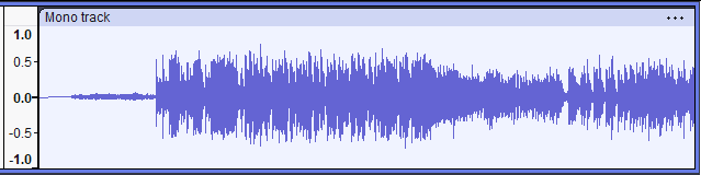
Waveform view of an audio track. In the waveform above, you can see the dynamics of a full song – softer intro on the left, then a much louder section with dense instrumentation (the thick blocky area in the middle), and fluctuations in energy throughout. This representation is intuitive: it’s basically what a microphone “hears” over time. But it doesn’t tell us directly which frequencies are present.

From Time to Frequency: The Spectrogram: Human ears and brains subconsciously do a form of spectral analysis – we can tell a bass guitar from a flute because of differences in frequency content. A spectrogram is a visual representation of audio in the frequency domain. It’s like a 3D graph: time on the horizontal axis, frequency on the vertical axis, and amplitude represented by color intensity (often brighter or warmer colors for higher intensity). We obtain a spectrogram by applying the Short-Time Fourier Transform (STFT) to the waveform, chopping the audio into small time frames and computing the frequency spectrum for each frame. The result looks like a heatmap of sound.

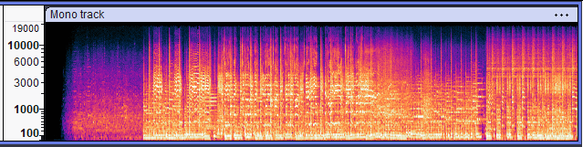
Spectrogram of the same audio track, showing frequency (vertical axis in Hz) over time, with color indicating energy. In the spectrogram above, low frequencies (e.g., bass and kick drum) are near the bottom, high frequencies (cymbals, vocal “s” sounds) are near the top. Bright horizontal bands might indicate a sustained note at a particular pitch; vertical streaks often indicate drum hits (which spread energy across many frequencies briefly). Notice how the spectrogram provides a lot more detail on the timbral content of the music: you might literally see the kick drum pattern as a series of thumps down low, or a vocal melody as a wavy line in mid-high frequencies.

For a broader look at how these concepts shape the production side of hip-hop, check out How to Improve Your Rap Flow and Delivery.

Why do we care? Because source separation can happen in either domain. Traditional methods and many modern ones (like Spleeter) operate on the spectrogram: they try to mask or separate the frequencies belonging to each source. Other methods, like Demucs, operate in the time domain: they try to directly predict waveforms of each instrument. Both approaches have pros and cons, which we’ll explore in depth. For now, just remember: a waveform tells us “when” something happens and how loud it is, while a spectrogram tells us “what frequencies” are present at each moment.

Why use spectrograms?
Some source separation methods (like Spleeter) operate in the spectrogram domain. They attempt to assign each pixel of the spectrogram to a source (vocals, drums, etc.). It’s often easier for a model to work on a spectrogram “image” because patterns like harmonics are clearly delineated in frequency, and the model doesn’t need to learn to separate phases.

Phase: An important but tricky aspect. Audio signals have not just magnitude (loudness at a frequency) but also phase (the alignment of the wave cycles). Human hearing is less sensitive to phase than magnitude, so many separation algorithms (e.g., Spleeter) ignore phase and work only with the magnitude spectrogra】, then later combine the result with the original phase of the mix. This can introduce some errors or artifacts, but it’s a common approach because predicting phase is hard. Demucs, by working in waveform, inherently handles phase.

Channels: Audio can have multiple channels (stereo = 2 channels). In stereo, sounds can be panned between left and right. Some separation clues come from stereo differences (for example, if vocals are dead-center and a guitar is panned right, an algorithm can use that info to help separate vocals from guitar by looking at commonalities/differences in L vs R channels). This is called spatial cues. Classic separation methods sometimes used simple tricks like “take the left channel minus right channel to remove center vocals” (vocal remover karaoke effect), which works when vocals are exactly in the middle and instrumentation is spread – but it’s crude and often nukes other content. Modern AI separation handles stereo in a learned way.

Stems vs Masters: In studio terms, stems usually refer to submixes or isolated instrument tracks from the multitrack recording session. What Spleeter and Demucs produce are estimated stems from the stereo mix. They won’t be as pristine as true studio stems, but they can be remarkably close (especially Demucs’s results for some instruments).

By understanding waveforms and spectrograms, you’ll better appreciate what these models are doing. Spleeter essentially looks at a spectrogram and decides, pixel by pixel, which instrument it belongs t】. Demucs looks at the raw waveform and tries to carve out new waveforms for each instrument such that when you add them up, you get the original wavefor】.

To summarize:

• Audio waveform: time vs amplitude; what we hear in time domain.
• Frequency spectrum: the recipe of frequencies that make up the sound at an instant.
• Spectrogram: spectrum over time, an image representation of sound.
• Source separation models may work in time-domain (on waveforms) or frequency-domain (on spectrograms). Each approach has pros/cons which we’ll soon explore.

With these basics covered, we can now comfortably discuss how Spleeter and Demucs approach the task. When we say Spleeter uses a “U-Net on spectrograms” you’ll know that means it’s treating the separation like an image segmentation problem on the spectrogra ​github.com】. When we say Demucs works in “waveform domain with Conv-TasNet”, you’ll understand it’s directly handling the raw wave and likely optimizing some notion of waveform erro】. These differences stem from the fundamentals we just reviewed.

What is a Stem?

Throughout this article we keep saying “vocals stem”, “drum stem”, etc., so let’s clearly define stem in this context. A stem is an isolated audio track of an individual instrument or group of instruments from the mix. If you have the stems of a song, you essentially have the multi-track session bounced into a few key submixes.

For example, consider a typical pop song. We could define stems as:

• Vocals stem – all the vocals (lead, backing, harmonies) mixed together, no instruments.
• Drums stem – the full drum kit mixed (kick, snare, cymbals, percussion).
• Bass stem – the bass guitar or synth bass.
• Other stem – everything else (guitars, keyboards, strings, etc.) mixed together.

If you play all those stems simultaneously at their original volume, you reconstruct the full son】. Stems are essentially additive components of the mix.

Why group instruments? It’s practical. While one could aspire to separate every instrument individually, that’s far more difficult and usually unnecessary for common use cases. So, separation systems focus on a few broad categories:

• 2 stems: Vocals vs Accompaniment (where accompaniment = “everything that’s not vocals”). This is great for karaoke or vocal extraction tasks.
• 4 stems: Vocals, Drums, Bass, Other. This became a de facto standard due to the MUSDB18 dataset which provides thos】. It covers the main elements in many genres.
• 5 stems: Some systems (like Spleeter’s 5-stem model) add Piano as a separate ste】, since piano often has a distinct role (and frequency range) in certain music.
• 6 stems or more: Research is exploring splitting “other” further – e.g., separating guitars and keyboards apart. Demucs’s team even tried a 6 stem model (vocals, drums, bass, guitar, piano, other】, though with mixed success on the new stems.

In the professional realm, when record labels talk about “stems for remixing”, they might provide stems like: Vocals, Drums, Synths, FX, etc., tailored to the specific track. Our AI tools have to decide categories without context of a specific song, so they use general ones (vocals, bass, etc. cover most songs).

So, a vocal stem from AI separation means ideally all vocals and only vocals. A drum stem means all percussion elements isolated. In practice, sometimes a stem might still have a hint of other instruments (imperfections in separation), but that’s the intent.

Stems are useful because they let you remix. If you have stems, you can mute one (removing that part from the song), solo one (hear it alone), or rebalance (make the vocals louder, etc.). Many classic albums have been remixed or remastered by going back to the stems (or multitracks). Now AI is enabling a similar approach even when you don’t have the multitracks.

One should note the difference between stems vs channels. A stereo song has 2 channels (left/right), but that’s not separating instruments, it’s just spatial distribution. Stems are about distinct instruments or groups, regardless of panning.

When you use Spleeter or Demucs:

• In 2-stem mode: you’ll get two files: typically named vocals.wav and accompaniment.wav. The sum of those equals the original song (after a tiny alignment, if any, and combining channels appropriately】.
• In 4-stem mode: you get vocals.wav, drums.wav, bass.wav, other.wav. Again, those sum to original (with minor differences if there were small errors). Each of these is stereo (because the original mix’s spatial cues for that instrument are preserved).
• In 5-stem mode (Spleeter only): vocals.wav, drums.wav, bass.wav, piano.wav, other.wav.

A question often asked: Do these tools separate backing vocals into the vocal stem? Yes – the “vocals” stem usually includes all vocal content (lead and backing). If the backing vocals are panned differently or treated with effects, the model doesn’t inherently split lead vs backing; it lumps all singing together. There are research efforts to separate lead vocals from backing vocals, but that’s a niche on niche. Most users just want all vocals together.

Another common question: Are stems stereo or mono? Typically, they’re stereo (to preserve the original stereo field). If the original had a guitar on the far left in the “other” stem, the separated other stem will have that guitar on the left. Demucs explicitly outputs stereo stems that sum to the original stereo mi】.

Instrument definitions:

• “Bass” usually means the bass instrument (bass guitar or synth bass). It doesn’t include bass drums; those go to drums stem.
• “Drums” includes all drums and cymbals, and often other percussive elements like hand claps, tambourine, etc., if present.
• “Other” is literally “whatever’s left after accounting for the above stems.” It tends to be midrange instruments like guitars, pianos (if not separated out), synths, strings, pads, etc. It’s the grab-bag category and often the hardest to define because it’s not homogeneous.
• “Accompaniment” (in 2-stem) = drums + bass + other all combined. Essentially the instrumental minus vocals.

Think of stems as layers in a musical parfait. The mix is the whole dessert; stems are the distinct layers you can spoon out individually. Spleeter and Demucs aim to recover those layers from the finished product.

To give an illustrative example: Take “Smells Like Teen Spirit” by Nirvana:

• Vocals stem: Kurt Cobain’s vocal track, isolated (verses more subdued, chorus screaming). You’d likely still hear a bit of the reverb or room ambience that was in the mix, but no guitars or drums except faint bleed.
• Drums stem: Dave Grohl’s drumming, the iconic drum intro clear as day, every fill isolated.
• Bass stem: Novoselic’s bass line chugging alone.
• Other stem: All the guitars (that dirty rhythm guitar and the layered power chords) together, possibly also the little guitar solo, etc., since there’s no “piano” or others in that track aside from guitar feedback etc., which would all be in “other.”

If you mute the vocals, drums, and bass stems and play only the “other” stem for that song, you’d basically hear just the guitars of Nirvana. It would sound like an instrumental minus rhythm section – thin but recognizable. If you instead mute the other stems and play just vocals, you’d get Kurt’s raw voice (which is a goosebumps experience for some – hearing the naked voice, complete with all its grit). That’s the power of stems: you can experience music in its component parts.

To a beginner: stems = instruments (in broad sense). You can think “the song separated into pieces.” It’s like having the multi-track faders at your fingertips. A decade ago, unless you were a studio insider, you almost never had that luxury. Today, an AI like Spleeter or Demucs brings you closer to that (though not perfectly).

Keep in mind that Spleeter and Demucs, by default, won’t separate two instruments that fall under the same stem category. If you have two guitars, both will be in “other” together. You can’t directly separate those two guitars apart with these tools (you’d need more specialized source separation or to treat it as a “two-source” separation problem where one guitar is “vocals” and the other is “other” or something hacky like that, which is non-trivial).

So, stems in this context are coarse categories, not every single instrument track. But those coarse categories cover the bases for most use cases (karaoke, remix, instrument practice, etc.).

Finally, note the difference between stems vs samples in music production lingo. Samples often refer to short clips or hits used in production, whereas stems refer to entire track components. Here we clearly mean the latter.

Understanding stems sets the stage for evaluating how well each tool does at isolating each part, and it will make it easier to interpret the evaluation metrics later (which are often reported per stem, like SDR for vocals, SDR for drums, etc.).

Difference Between Vocals, Accompaniment, Drums, Bass

When separating music, models typically distinguish between different source types. Let’s clarify these common source categories and why they’re distinct, both musically and in terms of what an algorithm “sees”:

• Vocals: This usually means the human voice – lead vocals and backing vocals combined. The human voice has a certain timbre and structure. In a spectrogram, vocals produce a series of harmonics (stacked horizontal lines at multiples of the fundamental frequency) that move when the singer sings different note】. Vocals also often sit in the mid-frequency range (say 100 Hz – 1 kHz fundamentals, plus sibilance up to 8 kHz). Vocals in studio mixes are often center-panned and dry (not too much stereo effect, at least for lead), which means in a stereo track, vocals are usually very correlated between left and right channels. This also gives a clue for separation: a voice often appears equally in both channels (since it’s center), whereas many instruments are spread. Culturally, vocals carry the lyrics and melody, so isolating them is high priority (for a cappellas or analysis of lyrics). Technically, vocals can be challenging because sometimes they overlap with instruments in frequency and time. But an interesting trait: humans have evolved to pick out speech and vocals even in noisy environments – our brains are good at it. We’ve essentially trained AI to do a similar thing.
• Accompaniment: This is a catch-all for “everything minus vocals.” In a 2-stem scenario, the model doesn’t try to distinguish instruments; it just lumps all non-vocal content. This actually simplifies the task: one neural network outputs vocals, the other outputs “background”. The background has a very different character from vocals – often more steady or percussive, usually not carrying linguistic information. Spleeter’s 2-stem model was trained to make this binary decision: voice or not voice. It’s presumably easier to train than a 4-way classification, which is partly why Spleeter’s vocal isolation via 2 stems can be a bit cleaner (fewer categories to confuse ​scite.ai】. The drawback is you can’t control drums/bass separately.
• Drums: Drums are percussive, producing short transient sounds with broad frequency content (a snare has a crack in mid-high freq, a kick has a thump in low freq, cymbals wash in high freq). In a waveform, drum hits appear as sudden spikes. In a spectrogram, they appear as vertical stripes (energy spread across frequencies at a given moment) rather than narrow horizontal lines. Also, drums (especially kick and snare) often have very distinctive envelope shapes. Demucs, for instance, leverages time-domain cues that a spectrogram approach might smea】. Another feature: drums (particularly kick, snare, toms) tend to be panned center in mixes, but cymbals and toms might be spread stereo. Also, drums usually repeat patterns. An AI can learn the pattern and thereby predict when a drum hit is part of the drum track versus say a strummed guitar (which has a different pattern). From a separation standpoint, drums often occupy unique transient patterns and often have less harmonic structure, making them, in some ways, “simpler” noise-like sources. Many classical source sep methods first tried to isolate drums (there’s an old algorithm called Harmonic/Percussive Separation that uses the fact that harmonics = horizontal lines (tonal), percussion = vertical lines (noise) to separate them). Spleeter and Demucs do this learning-based, but conceptually similar idea: one part of the network looks for noisier transient stuff = drum】.
• Bass: Bass refers to the bass instrument (electric bass, upright bass, synth bass). Not to be confused with “bass drum” (kick drum) which is drums. The bass typically occupies low frequencies (fundamentals often 40 Hz – 200 Hz). It also often has harmonics up to maybe 1 kHz (especially if the bass tone is rich or has string noise). Bass in spectrograms shows up as the lowest set of horizontal lines. One special thing: the bassline is usually monophonic (one note at a time) except in some complex music. That means its harmonics move in lockstep. A network can exploit that to identify bass. Also, in mixing, bass is usually center (for stereo compatibility) and often slightly louder relative to other content in low freq. Bass is tricky because it can overlap with the kick drum’s frequency. Sometimes separating kick vs bass is a challenge – an algorithm might lump the kick’s thump into the bass stem or vice versa. Demucs’s original paper noted that with enough training data, it even beat the “ideal ratio mask” for bass, meaning it did an exceptional job separating bass without letting kick blee】. Bass lines often have a smoother, more tonal quality than drum hits, which helps differentiate. From a use perspective, bass stems are great for musicians wanting to transcribe or learn bass parts, or for remixers maybe to remove the bassline and add their own.
• Other: This is everything that doesn’t fall into the above. It could be a single dominant instrument (like in a power trio rock, “other” is mostly electric guitar), or a mishmash (in a pop song, “other” might include guitars, synth pads, pianos, strings all together). Because it’s a mixture of multiple instruments, “other” is the hardest stem to separate cleanly. Typically, it has a lot of mid-range content (500 Hz – 8 kHz from various instruments). Often instruments in “other” have harmonic structure but overlap each other. AI sometimes struggles here: e.g., a piano and a guitar playing together – separating them apart is beyond current models, so they live together in “other.” That means the “other” stem is often the messiest or most artifact-prone, and also usually has the lowest SDR in evaluation】. Still, it’s useful – if you remove vocals, drums, bass, whatever remains is usually the melodic and harmonic backing, which can be used as an “instrumental minus rhythm section” or for sampling chords, etc.

Why treat these categories separately?
Because each has distinct characteristics that a model can specialize in. Spleeter literally trained separate U-Nets for each ste】 (or a combined network that outputs multiple masks – but effectively, it has separate mask outputs for each source). Demucs has one model that outputs all sources simultaneously, but internally, certain layers or features may be tuned to certain sources (and in the latest Demucs, they even fine-tune each source output individually with specialized models to boost qualit】).

Also, metrics are measured per stem because performance can vary widely by stem. For instance, as the Spleeter paper shows, bass tends to have lower SDR than vocals or drums for many method】 – likely because bass is low freq and gets masked by kick or lacks high-frequency detail to latch onto.

Instrument Frequency Ranges (approx):

• Vocals: 100 Hz (male low) / 200 Hz (female low) up to ~1 kHz fundamentals; harmonics to 8 kHz and sibilance up to ~10 kHz.
• Drums: Kick ~50–100 Hz thump; Snare ~150–250 Hz body + 3–6 kHz snap; Hi-hat/Cymbals ~5–15 kHz; Toms various. But drums are broad.
• Bass: 40–60 Hz low E (or low B on 5-string ~31 Hz) up to maybe 500 Hz fundamentals, with some overtones higher.
• Other: Guitars ~80 Hz (low E) – 1 kHz fundamentals, harmonics higher; Piano spans entire range 27 Hz to ~4 kHz fundamentals; Synths can be anywhere; etc. “Other” is broad midrange usually.

So you see, these categories carve up the spectrum somewhat:

• Bass mostly low.
• Drums span low (kick) to high (cymbals) but are transient.
• Vocals mid & some highs, harmonic.
• Other mid & highs, harmonic (but more steady/continuous or polyphonic than vocals usually).

This division of labor makes the separation task tractable.

Political/Personal Note: Vocals are often considered the most “protected” part by labels (they carry the identity of the song), yet fans are most eager to extract vocals to either enjoy alone or remix. Instruments (drums/bass) are sometimes available via official instrumentals, but vocals rarely are. Thus, vocal stems extraction is very culturally significant – allowing fans unprecedented access to the heart of the song.

One more subtlety: sometimes backing vocals or ad-libs might be quiet or panned – models can miss those or put them partly into “other.” Overall though, they aim to capture any vocal-like audio in the vocal stem.

So to recap:

• Vocals = any singing/rapping voice content.
• Drums = the percussion elements.
• Bass = the bassline instrument.
• Other = the rest (guitars, keys, pads, etc.).

It’s a pragmatic grouping that covers most use cases.

Understanding these differences will also help in later sections where we examine how well each tool handles each category. For instance, if we find Demucs has 10.8 dB SDR on drums vs Spleeter’s 6.7 d】, we’ll know why (drums transients, etc., Demucs time-domain strength). Similarly, we’ll see how vocals are handled by each.

Think of a song as a puzzle with four big pieces (vocals, drums, bass, other). Source separation is about reassembling those pieces. Each piece has a unique shape (characteristics) that the algorithms are designed to recognize. Now, with that mental model, we can move on to see how Spleeter and Demucs tackle that puzzle differently.

Background on Spleeter

In late 2019, Deezer – a French music streaming company – surprised the Music Information Retrieval (MIR) community by open-sourcing a tool called Spleeter. It wasn’t the first source separation algorithm, but it was the first to achieve wide adoption, for a few reasons:

• It was free and open (MIT License).
• It came with pre-trained models that were easy to use.
• It was simple to install (a pip package) and could run on modest hardware.
• It was fast – able to separate audio much faster than real-tim】, which was a game-changer.

The Origins: Spleeter was developed by researchers at Deezer (Romain Hennequin and team). Deezer’s interest was partly to help MIR tasks – if you can separate vocals, you can do lyric transcription or melody extraction more easil】. There was also likely a practical interest for karaoke or remix features on their platform. They published a short paper (in JOSS, 2020) describing Spleete​ scite.ai】.

Key points from Spleeter’s design:

• It is built on TensorFlow (1.x at the time, later made compatible with TF2). This made it relatively straightforward for many to run (since TF had widespread support and could use GPUs).
• It uses an encoder-decoder (U-Net) convolutional neural network operating on the spectrogram of the audi ​github.com】.
• It outputs a mask for each source, which is applied to the input spectrogram to get the separated source spectrogram】.
• The output spectrograms are then converted back to audio via inverse STFT, using the original phase and optionally a multi-channel Wiener filter for refinemen】.
• They provided models for 2, 4, and 5 stems. The 4-stem model (vocals, drums, bass, other) became the most widely used default.

In training, Spleeter used Deezer’s internal dataset of isolated tracks (they mention the Bean dataset】. Notably, they did not train on the public MUSDB18, yet when tested on MUSDB18, Spleeter’s performance was near state-of-the-art of that tim】. This was impressive: it showed good generalization.

Spleeter’s 4-stem model structure:

• It’s a 12-layer U-Net (6 down, 6 up】. Downsampling presumably halves the time dimension or frequency dimension per layer (they followed a prior paper’s spec, likely Jansson et al. 2017 which downsampled frequency).
• At each layer, it likely doubles the number of feature channels, then the decoder mirrors it.
• Skip connections join each down layer to the corresponding up layer, allowing fine details to bypass the bottleneck.
• Each source has its own mask output. They probably train one big network with multiple outputs (instead of separate networks per source) – this way the network can learn to allocate energy between sources in a coordinated way.
• Loss function: they used an L1 loss on spectrogram magnitudes (between estimated and true source spectrograms】. They also tried multi-channel Wiener filter as a post-process, which isn’t learned but improves SDR a bit by optimizing the distribution of energy between estimated sources given the mixture.

Why U-Net? The U-Net architecture was borrowed from image segmentation, and it had been used successfully in singing voice separation (a 2017 paper by Jansson et al. used a U-Net for separating vocals from mix). U-Net’s strength is combining global context (via downsampling) with local detail (via skip connections). For audio spectrograms, global context helps distinguish sources (like understanding the overall harmonic series), and local detail ensures things like onset times and precise frequencies are captured.

Performance: Spleeter’s claim to fame (besides being open) was its efficiency. They reported 100× real-time speed on GPU for 4 stem】. Technically, this is due to the fully-convolutional nature of the network and using a high-level language (C/C++ in TF backend) to perform the heavy FFTs and convolutions. This made it feasible to separate dozens of songs quickly, which was previously painful.

The name “Spleeter” is presumably a play on “splitter” with a French accent or something fun. It quickly became a meme in producer communities – “just Spleet it out” people would say when wanting an a cappella.

Community Impact: Within weeks of release, Spleeter had thousands of stars on GitHub​ github.com】. It lowered the barrier for many hobbyists to use source separation. Before that, one had to either compile research code or use slow proprietary software. With Spleeter:

• Mashup artists on YouTube started pumping out more a cappella/instrumental mixes.
• Indie game developers used it to strip vocals from songs for rhythm games.
• The MIR research community appreciated having a baseline model to use for tasks like chord recognition on separated stems, etc.

Deezer’s motivation was partly altruistic: “to help the MIR community leverage source separation】. They believed the tech had matured enough to be useful. Indeed, Spleeter’s quality wasn’t perfect, but it was good enough for many use cases, and ease-of-use meant people actually used it widely.

One might wonder: Did Spleeter end up in Deezer’s app for any feature? As of my knowledge, not directly in the user-facing streaming app. It seems more like a contribution to the research/open-source world (and to get kudos in tech press). But its open-source release arguably nudged the field forward – by mid-2020s, several other companies and researchers open-sourced strong models (Facebook with Demucs, ByteDance with their Separation challenge contributions, etc.). It became a bit of a friendly competition.

Limitations of Spleeter (background): Spleeter’s design choices, while practical, impose some limits:

• Being spectrogram-based, it doesn’t handle phase. This can lead to some metallic sounds or whooshes (artifact).
• The model was trained up to 11 kHz frequenc】, which implies it might not fully capture very high “air” frequencies in sources (they probably cut off spectrogram above 11 kHz to reduce size, since a lot of musical energy is below that). That means separated stems might lose a bit of the extreme treble. In practice, you rarely notice, but it’s a design decision.
• It uses TensorFlow, which some in 2025 might find old-fashioned as PyTorch became more popular in research. But for end users, that doesn’t matter much.
• Spleeter wasn’t really designed to be fine-tuned on your own data easily (though they did allow training; but you need your own isolated tracks which most users don’t have, so they just use pre-trained).
• As of 2025, Spleeter has not had major updates since 2019 release (no Spleeter v2 with better quality). Meanwhile, other models surpassed it in quality.

But despite these, Spleeter remains a workhorse. It’s stable, predictable, and fast. It’s rather “polite” in how it separates – meaning it usually doesn’t introduce weird artifacts that draw attention, it more often just leaves some bleed or dulls some part.

One measure in their paper: they compared Spleeter’s metrics to other models like Open-Unmix and the original Demucs (v1). Spleeter was “almost on par with Demucs” in SD】, which is impressive given Demucs v1 was state-of-art at the time. They noted Spleeter actually achieved higher SIR (less interference) for vocals than Demucs, at the expense of slightly lower SAR (more artifacts】. That hints at Spleeter’s approach: aggressively mask out non-vocal content (giving high SIR), but the masking can cause artifact (lower SAR). Demucs left a bit more bleed (lower SIR) but sounded more natural (higher SAR). We’ll revisit this in comparison sections.

As Greg Kot might note, Spleeter’s open approach was somewhat punk rock in the research world – they didn’t fuss about absolute perfection, they just threw it out there for people to use, with a “DIY” spirit. And the community ran with it. In doing so, Spleeter probably collected more real-world testing hours than any previous separation model.

To sum up Spleeter:

• Who made it: Deezer (a streaming service’s research team).
• When: Released open-source in November 2019.
• What it is: A fast, easy, CNN-based source separator working on spectrograms, with pre-trained models for 2/4/5 stems.
• Why it matters: It popularized AI source separation, making it accessible outside specialist circles.

As we proceed, remember that Spleeter represents the spectrogram masking paradigm – it treats separation somewhat like image filtering. It’s effective and efficient, but has inherent limitations (phase issues, limited frequency resolution). Demucs will represent a different paradigm (waveform modeling).

One more note: The name Spleeter became almost generic – people often refer to any AI separation as “Spleeter” in casual talk, even if using a different model. That’s how influential it was, akin to how “Photoshop” became a verb. Now that we have Spleeter’s background, we can dive into Demucs, which has quite a different story and philosophy.

Background on Demucs

At the same time Spleeter was making waves, Facebook AI Research (FAIR) was working on pushing the envelope of separation quality with a model called Demucs. Demucs stands for “Deep Extractor for MUSic Sources” or something along those lines (the original paper doesn’t explicitly define the acronym, but presumably “DEep MUltichannel Source separation” or simply a stylish take on “mucs” for music). For an even deeper look at Demucs, check out Demucs – A Deep Dive Into the Ultimate Audio Source Separation Model.

The Genesis: Demucs was introduced in a 2019 arXiv pape】 by Alexandre Défossez et al. The key idea: instead of operating on spectrograms like most other methods, Demucs would operate directly on the waveform (time domain). This was inspired by a then-recent success in speech separation called Conv-TasNet (Luo & Mesgarani 2018), which worked in time domain and achieved great results for speech. The authors adapted Conv-TasNet to music, and also proposed their own architecture – Demucs – which incorporated ideas from both Conv-TasNet and Wave-U-Net, plus an LSTM for sequence modelin】.

Demucs v1 (2019):

• It uses an encoder-decoder convolutional network on the waveform with a U-Net structure (skip connections) and a *bidirectional LSTM bottleneck】.
• The waveform is input as stereo (2 channels) and the model outputs 4 waveform signals (stereo stems for each source).
• The encoder part is like a series of 1-D convolutions with stride >1 to downsample the time resolution while increasing feature channels (similar to how a Wave-U-Net works, or like how MP3 encoding splits into subbands). The decoder does the reverse with transposed conv (aka deconvolution).
• The LSTM in the middle allows the model to capture long-term dependencies. Music has structure (verses, choruses) and sometimes something that happens later can inform separation earlier (like recognizing an instrument’s timbre when it plays solo might help separate it in sections where it’s mixed with others).
• They train Demucs with an L1 loss on waveform directl​ arxiv.org】 (or a combination of time and STFT loss, I recall they experimented but found time L1 robus​ arxiv.org】). This means they’re telling the model: “produce a time signal whose samples match the ground truth source’s samples.”
• Demucs v1 was already good: on MUSDB18, it achieved ~6.3 dB SDR average, beating many spectrogram models of the tim】. However, it had some “bleed” issues – e.g., some vocals leaking into the other stem, etc., which they noted in the paper (they did a human eval where people noticed slight interference】.

Facebook open-sourced the code for Demucs (first via torch.hub in 2019, then proper GitHub repo). Initially, Demucs v1 was not as wildly adopted as Spleeter, likely because:

• It was heavier to run (PyTorch, not as optimized for speed).
• It wasn’t as plug-and-play for casual users then (though torch.hub made it relatively easy for Python folks).
• But researchers and audio tinkerers definitely noticed it because of the quality jump.

Demucs v2 and v3 (2020-2021): Défossez didn’t stop. He iterated:

• Demucs v2 (mid-2020): Minor improvements, possibly training on more data or using better data augmentation. Also a “quantized” version (smaller model, 8-bit weights) was provided for those who want faster inference with slight quality tradeoff. They might have also made it friendlier (packaging etc.).
• Demucs v3 (aka “Hybrid Demucs”) (2021): This was a big update. They introduced a hybrid time-frequency approac】. Hybrid Demucs processes audio in two branches: one branch is the time-domain CNN (like earlier Demucs), another branch processes a spectrogram (magnitude) with a small CNN. The two are combined inside the network. This way, it can leverage advantages of both domains. They also increased model capacity and trained on the augmented dataset MUSDB18-HQ (a higher-quality version of MUSDB with 150 extra songs】. The result: Demucs v3 significantly improved separation quality (approx 7.0+ dB SDR). It won the top ranks in the 2021 music separation challenge (ISMIR MusDemix challenge).
• Demucs v3 also introduced a 6-source experimental model (with guitar and piano stems separate) and a more efficient variation (they dropped the LSTM in one variant in favor of Temporal Convolutional Networks, etc.). They also introduced the concept of fine-tuning separate models for each source after training the main model (so-called “source-targeted models”) to eke out extra performance.

Demucs v4 (Hybrid Transformer Demucs) (2022): The latest iteration combined Demucs v3 with Transformers:

• They replaced the LSTM (or the center of the U-Net) with a Transformer Encoder that operates across both time-domain and frequency-domain representation】. This cross-domain attention allowed the model to globally reassign information between the waveform and spectrogram views of the signal.
• They also implemented a form of sparse attention to increase receptive field without huge compute, and did per-source fine-tuning. The best variant (“HT Demucs FT + sparse”) reached ~9.2 dB SDR average on MUSDB18, which as of 2022 was state-of-the-ar】.
• They mention training on an internal dataset of 800 extra songs on top of MUSDB-H】 – so by now, Demucs had seen a ton of varied data.
• Demucs v4 was released in 2023 on GitHub (and via PyPI), but with caution that it’s not actively maintained by Meta anymore (Défossez moved to another org, but he still tends to the open repo occasionally).

It’s worth noting the philosophical difference in approach:

• Spleeter focuses on practicality: good-enough quality, super fast.
• Demucs focuses on pushing quality: willing to increase model complexity and computation to minimize artifacts and bleed. It leverages heavy deep learning machinery (LSTMs, Transformers).
• Spleeter uses a divide-and-conquer frequency masking approach. Demucs uses a generate-and-predict approach in time domain.

Community & Usage: Initially, Demucs was mainly used by the more tech-savvy folks (people who didn’t mind running Python scripts). As Demucs v3/v4 arrived, its quality lured more users, and friendly forks and GUIs came: e.g. the Ultimate Vocal Remover (UVR) package included Demucs models with a simple interface, so many non-coders started using Demucs through that, for tasks like vocal removal or drum extraction. By 2023, Demucs had become the go-to for those who prioritized quality. For example, mixing engineers playing with unofficial remixes, or archivists isolating tracks for remix projects, would often try Demucs because it generally sounds cleaner.

Demucs stands on the shoulders of giants: It borrowed from Conv-TasNet (the idea of a learned encoder and mask in time domain) and from Wave-U-Net (the U-Net structure in time). It combined that with sequence modeling (LSTM/Transformer) which is like giving the model some memory or foresight. This memory aspect is something Spleeter lacks – Spleeter’s U-Net sees only a limited context around each time-frequency point (maybe a few seconds at most, due to CNN receptive field). Demucs’s LSTM/Transformer can potentially consider the entire song when separating any given moment, helping maintain consistency (e.g., an instrument’s tone stays consistent across the track separation).

One anecdote: The original Demucs paper’s title bragged that with extra training data, Demucs could even beat the “oracle” mask for bas】. The “oracle” mask means if you had perfect knowledge of the isolated sources’ magnitudes but not phase, what’s the best you could do. Demucs exceeded that for bass – implying it was capturing something beyond just magnitude cues (likely phase/time structure), which is a big win for time-domain method.

Another unique pro of Demucs: because it reconstructs waveforms, the separated signals often have a more natural sound (phase-coherent, proper transients). Spleeter’s outputs sometimes feel a little alien or “disembodied” due to phase issues. Demucs outputs, when you solo them, could fool you into thinking they might be real instrument recordings (except when there’s obvious bleed of something faintly in background).

It wasn’t all rosy: Demucs’s complexity means slower speed and more memory. Also, early versions had slight noise issues (some users reported Demucs added a faint hiss or “buzz” during silent part】 – possibly due to attempting to reconstruct background noise that original mix had or the way loss was optimized). But these were minor compared to the leap in quality.

Meta’s approach vs Deezer’s reflects a difference in goals: Meta was aiming for SOTA research (hence Transformers and big training), whereas Deezer was aiming for a useful tool. The tones of their releases were different: Spleeter: “here’s a tool, have fun,” Demucs: “here’s a novel architecture, see our SDR scores.” Over time, though, these lines blurred because Demucs also became packaged for fun use, and Spleeter contributed to research by being a baseline.

In summary, Demucs’s background:

• Developed by a major AI lab aiming for high-quality separation.
• Evolved through multiple versions, each improving quality significantly.
• Open-sourced (MIT License as well) and by v4 became arguably the top open model for music separation.
• It validated that time-domain approaches can outperform frequency masking ones, breaking a long-held assumption in audio that “you separate in frequency domain.”

Now, having backgrounds on both Spleeter and Demucs, we have the context to compare them in detail: from how their architectures differ to how that affects performance, to usage differences, etc. Think of Spleeter as a family sedan – reliable, fast, gets you there – and Demucs as a high-end sports car – higher performance but more finicky and resource-hungry. Both can drive the route; each has its style.

Model Architectures Explained Simply

Let’s break down the architectures of Spleeter and Demucs in (relatively) simple terms, drawing some analogies to help conceptualize them.

Spleeter’s Architecture (U-Net on Spectrograms):
Imagine you have a spectrogram of a song (an image showing frequencies over time). Now, suppose you want to “color” each pixel of this image with a label: red for vocals, green for drums, blue for bass, yellow for other. If you could do that perfectly, you’d essentially separate the sources, because you’d know which time-frequency components belong to which source. For a taste of the behind‑the‑scenes of mixing and remixing, explore Rap God: Rap Unraveling Eminem’s Iconic Masterpiece.

Spleeter’s approach is akin to an image segmentation task on this spectrogram. It uses a U-Net convolutional neural network to produce, for each source, a mask that ranges 0–1, indicating how much of the energy at each time-frequency point belongs to that sourc】.

• A U-Net is shaped like the letter U: an encoder (downsampling path) compresses the image into a low-resolution representation capturing high-level info, and a decoder (upsampling path) reconstructs an output of the original size (here, the masks​ github.com】. Skip connections directly link encoder layers to decoder layers of the same size, providing a shortcut for fine details.
• For example, Spleeter’s encoder might take the input spectrogram of shape (frequency_bins × time_frames) and first apply conv/pooling to halve the frequency resolution, capturing broad spectral patterns. It goes down 6 layer】, each time aggregating more context (so the bottom layer’s “view” might be, say, one that covers the entire frequency range in coarse blocks and a couple seconds in time – capturing something like “there is a voice harmonic series here, or a drum hit pattern here”).
• The decoder then uses this condensed knowledge to build masks. The skip connections feed in the original fine detail from the encoder’s corresponding levels, so the output mask can align precisely to actual features in the input.

Think of the encoder as analyzing the mix: “okay, I see harmonic stripes (could be vocals or guitar), I see broadband bursts (drums), I see low steady tones (bass).” The decoder then says “let me paint an output for vocals: highlight the harmonic stripes that match human voice characteristics; for drums: highlight those bursts; for bass: highlight the low steady tones,” etc. It follows whatever it learned from training on how to differentiate these patterns.

Mathematically, inside Spleeter:

• The input is typically a complex spectrogram, but they likely feed the magnitude (and maybe duplicate for both channels or treat channels as separate input channels).
• The output for 4-stem is four masks (each the same dimension as input spectrogram).
• They apply each mask to the mixture spectrogram to get estimated source spectrogram】.
• Then invert each via ISTFT using mixture phase, and optionally refine with Wiener filter.

A concrete example: At a moment where a vocal note and a guitar note overlap at the same frequency, Spleeter’s U-Net looks at context: maybe it sees formant structure or vibrato indicating voice, vs the guitar’s more static harmonic. It might assign more mask weight to vocals at that frequency if it’s confident. If uncertain, it might split energy or leave some in both.

The U-Net is fully convolutional, meaning it uses learned filters (like small patches scanning across time-freq). These filters can detect things like “vertical line = drum hit” or “horizontal ridge = sustained note.” The deeper layers detect combos (“multiple parallel horizontal lines = vocal or instrument with rich harmonics”).

Demucs’s Architecture (Waveform Conv-TasNet + LSTM):
Demucs works in the time domain, so think in terms of waveform oscillations. A raw audio waveform is like a very fast squiggly line. Separating sources in time domain is like trying to carve that squiggly line into multiple squiggles that add up to it.

Picture you have multiple musicians playing, and their waveforms add together. Demucs tries to learn to subtract out each instrument’s waveform from the mix. One way to do that: use a bunch of learned filters that can transform the waveform into an intermediate representation where sources are more separable. Conv-TasNet does this: it learns a filterbank (like an adaptive Fourier Transform】. Demucs similarly uses convolution layers to progressively transform the time signal.

The encoder part of Demucs might do something like:

• First layer: a 1-D convolution with, say, 8 ms kernel, producing 100 feature channels, stride maybe 4 ms. This might break the waveform into 100 “subsignals” each at 1/4 the time resolution. These could be analogized to frequency subbands, but they are learned so they could also encode other patterns.
• Subsequent layers: further downsample (maybe next layer stride 4 again, now each step is 16 ms, etc.), increasing feature count. After 5-6 downsamples, you have a very compressed representation (low temporal resolution, high feature depth). This is the encoder output.

Think of the encoder as a set of ears tuned to different things: one filter might pick up kick drum thumps (a low frequency oscillation pattern), another might pick up snare attacks (a sharp transient shape), another might resonate with human voice pitch patterns, etc. By the time you get to the bottom, the combined pattern of activations in those feature channels encodes which sources are present and with what characteristics.

Now, Demucs adds a bidirectional LSTM at this bottlenec】. That means it takes the sequence of encoded frames (downsampled time steps, maybe each representing ~100 ms of audio or something after several downsamples) and processes it forward and backward. This gives the model memory of what came before and after. The LSTM can carry info like “the instrument playing now is the same guitar that was playing a few seconds ago” or “there’s a vocal starting here and continuing for next 10 seconds.” Essentially, it can enforce consistency over time and use future context to decide separation in the present (non-causal, since for offline separation we don’t mind using future info).

After the LSTM, the decoder part mirrors the encoder: transposed conv (a learned upsampling) to reconstruct the signals. Skip connections likely exist here as well (Demucs paper said “with skip U-Net connections​ ai.honu.io】). So features from encoder layers feed into decoder layers to help reconstruct finer details that were too fine for LSTM to care about.

The decoder outputs, ultimately, waveforms for each source. How? The final layer might output (N_sources × N_channels) feature maps that are the same length as the input audio (through iterative upsampling). They train it such that each of those outputs matches the ground truth source signal.

Another perspective:

• Spleeter outputs masks (weights) for spectrogram, so it’s inherently a “filtering” approach.
• Demucs outputs actual signal estimates. It’s constructing new waveforms sample by sample (though using context). In a sense, it’s generative – it creates the source signals from scratch such that they sum to the mix (they ensure that by a mixture consistency loss or simply by learning, not 100% but demucs does tend to nearly sum to original).

Simplified analogy:

• Spleeter is like a chef with a spice rack, tasting a soup (the mix) and deciding which ingredient’s flavor (freq component) to reduce or enhance to isolate tastes. They work in the “frequency domain” of flavor.
• Demucs is like a group of drummers trying to transcribe a drum ensemble performance by ear, each drummer picks out their own rhythm from the complex sound and plays it (reconstructing in time). In doing so, each drummer’s part when played together recreates the whole performance. This is done in the time domain.

One big advantage of Demucs: by working with waveforms, it naturally deals with phase. It can align wave cycles properly and handle transients precisely in time. Also, Demucs can learn to exploit subtle phase differences between stereo channels to separate sources that overlap in frequency (something Spleeter’s magnitude masks can’t fully do).

Conv-TasNet portion: Demucs’s encoder/decoder is similar to Conv-TasNet’s analysis & synthesis filterbanks, except Demucs’s are multi-layer with skip connections (more complex than TasNet’s single-layer basis). Conv-TasNet also used a temporal convolution stack (a bunch of dilated convs, like WaveNet) instead of LSTM for context. Demucs chose LSTM (v1) and then Transformers (v4) for context modeling.

Why LSTM/Transformer? Because music has structure and long-range correlations. For example, if no vocals have been present for a minute, when something voice-like appears, the model might confirm it’s vocals by noticing lyrical content or typical voice range that extends beyond a short window. Or if a certain guitar tone is identified in a solo, the model can then better isolate that guitar when it’s mixed with other instruments. The LSTM can carry that “guitar tone signature” across time.

Hybrid Demucs (v3) adds a small spectrogram branch, basically giving the model a “spectrogram view” as well, likely to catch things like high-frequency details or certain patterns easier seen in freq domain.

Transformer in v4 basically allows each time step’s representation to attend to all time steps and all frequency bins representation, crosslinking information. The cross-domain transformer effectively says “hey time-domain feature, check with frequency-domain feature whether this pattern is voice or not” and vice versa.

So structurally:

• Spleeter: CNN (2D) -> 4 output masks.
• Demucs: CNN (1D) + RNN -> 4 output signals.
• Demucs uses more parameters and compute (the LSTM alone has a ton of parameters, Transformers even more).
• Spleeter’s number of parameters is relatively small (maybe on order of 20 million). Demucs v4 probably hundreds of millions (with transformer layers).

Training Regimen:

• Spleeter trained on internal data but interestingly not on MUSDB (so no overfit to test). It used augmentation (they mention none explicitly besides maybe random gain).
• Demucs v1 trained on MUSDB train + extra 150 songs with heavy augmentation (pitch shifts, etc.】. v4 on a much bigger set. They also sometimes train in multiple stages (pretrain on one set, fine-tune on another).
• Loss: Spleeter used spectrogram L1. Demucs v1 used waveform L1 + some STFT loss trials, v3/v4 included multi-resolution STFT loss (common technique to improve perceptual quality by ensuring frequency content matches as well as time) and had an additional “combination of L1 on time + L1 on spectrogram + maybe SI-SDR loss”.

Summary of architectures:

• Spleeter – Encoder/Decoder CNN on spectrogram. Think of it as an image-to-image network where input is a spectrogram and output is a set of soft masks (one per source) of the same size. It’s relatively shallow (12 conv layers) and uses skip connections heavily. It focuses on magnitude. The heavy lifting (ensuring separated audio sounds good) partly offloaded to using mixture phase at the end.
• Demucs – Encoder/Decoder CNN on waveform + sequence modeling. It’s like an autoencoder for raw audio, but multi-output. It explicitly generates waveforms for each source. It’s deeper and uses recurrent/attention layers to capture long context. It directly optimizes for time-domain signal match.

In car terms: Spleeter’s like an automatic transmission, easy to drive, but you don’t have manual control of phase etc. Demucs is like a manual transmission high-performance car, giving more control over the fine timing (phase) and fidelity, but requiring more skill (computation) to operate.

With architecture basics laid out, we can now understand many differences ahead: why Demucs might have better transients (time conv vs STFT bin smoothing), why Spleeter is faster (convs on smaller spectrogram vs huge convs on long waveform), why Demucs needs more RAM (storing long sequences vs smaller images), etc.

Spleeter Using U-Net

Spleeter’s core is the U-Net architecture applied to spectrograms. Let’s unpack what that means in a straightforward way.

U-Net Refresher: Initially developed for biomedical image segmentation, a U-Net has an encoder that progressively downsamples the image and a decoder that upsamples back to original size, with skip connections linking corresponding level ​github.com】. It’s called U-Net because if you draw it, the path down and up form a U shape. The skip connections ensure the decoder has access to high-resolution details from the encoder.

In Spleeter’s case:

• The “image” is a spectrogram slice. Actually, Spleeter likely processes the whole spectrogram at once or in large chunks. Possibly it treats the stereo channels as separate channels in the input (like a 2-channel image).
• It encodes that spectrogram via a series of conv layers.

Let’s imagine a simple scenario: We have a 1024-bin, 5-second spectrogram (with, say, 431 time frames at 11.6 ms hop). The U-Net encoder might:

• Conv Layer 1: 2D conv with stride (2,2) might reduce time resolution by 2 and freq by 2, output e.g. 16 feature maps. Now dimension ~512×215 in freq×time.
• Layer 2: another down: 256×108, more feature maps (say 32).
• … down to Layer 6: maybe ~16×3 or something, with many feature maps (say 256).

At the bottom, the network has a very compressed representation: it has combined information across frequency and time to identify broad structures.

For example, one feature map at the bottom might respond to “presence of a harmonic series pattern” (which indicates a tonal instrument or vocal). Another might respond to “percussive noise burst”. Essentially, the encoder is disentangling different elements present.

Now the decoder goes in reverse:

• Layer 6 decodes from 16×3 to 32×6 (just rough numbers, doubling each step).
• It uses transpose conv (learned upsampling) and adds the skip connection from encoder’s corresponding layer (which gives it precise localization cues).
• By the top, it returns to 1024×431 resolution.

However, the output isn’t a single spectrogram; it’s a set of masks. If 4 stems, the network outputs 4 channels at top (or possibly 8 channels – 4 stems × 2 channels, if it outputs both stereo channels for each stem, but likely it outputs masks for magnitude same for both channels, simpler assumption). So think of it as output of shape [4, 1024, 431] representing the estimated magnitude spectrogram for each source.

They apply these as masks on the original mixture spectrogram: S^i(f,t)=Mi(f,t)⋅X(f,t),\hat{S}_{i}(f,t) = M_{i}(f,t) \cdot X(f,t),S^i​(f,t)=Mi​(f,t)⋅X(f,t), where XXX is mix spectrogram, MiM_iMi​ is mask for source i output by networ】.

If using multi-channel Wiener filter (MWF), they’d take these estimated magnitudes and do a more complex algorithm to refine using mixture phase correlations – but that’s a separate step outside the network.

So, what is the U-Net learning? Essentially, it’s learning to detect patterns in the spectrogram that belong to each instrument and assign them to the right mask. It’s like partitioning the spectrogram. Because it’s data-driven, it figures out an optimal way to do so that minimizes error.

For example:

• Vocals have harmonics that usually extend in parallel lines. The U-Net can dedicate some part of itself to recognizing those and routing them to the vocal mask output. It might also pick up that vocals often occupy center stereo and have certain formant shapes (broad energy around 300–3000 Hz, etc.). If a vocal and guitar overlap, the network might use subtle cues (like slight differences in timbre or timing) to still separate them moderately well.
• Drums produce vertical streaks. The network can allocate vertical textures to the drum mask. If a drum hit coincides with a vocal sustain, the spectral shape is different (drum is broadband noise, vocal is narrowband harmonic). The U-Net likely has filters that detect broadband vs narrowband and accordingly subtract the drum portion from vocal mask and put it in drums mask. The result: a bit of drum sound still in vocal maybe (if it’s not perfect), but largely separate.
• Bass is identified by energy in low freq with usually a harmonic at maybe 2x, 3x frequency. Also bass lines often have repetitive patterns. But since the U-Net’s convolution filters likely slide over time, they can pick up periodicity. Alternatively, the network might somewhat rely on frequency range: below 100 Hz is mostly bass and kick. The model can decide to allocate steady tonal part to bass mask and leave the transient part (kick) to drums. If the kick is very tonal (808 kick with a decay), that can confuse it – sometimes Spleeter misroutes 808s because they are drum and bass hybrid.

The skip connections ensure that fine details like exact frequency of a vocal harmonic or timing of a drum hit are preserved into the output mask. Without skip connections, a coarse decoder might blur things. Spleeter’s output is fairly precise (if it identifies a vocal harmonic at time t, the mask will specifically emphasize those frequency bins at that time).

One can think of skip connections as: the encoder tells decoder “here’s roughly where things are and what general pattern they are,” and then skip provides “and here’s the fine-grain texture at those points.” The decoder uses both to carve out masks.

Mask Values: They’re typically between 0 and 1. They likely used a sigmoid at output to ensure that. And likely trained with a constraint that masks sum to 1 across sources (or at least encouraged that by combining losses】. Indeed, they mention multi-channel Wiener filter: that assumes initial estimates sum approximately to mix. To enforce that, they might have added a penalty if sum of masks deviates from 1 at each time-freq (some implementations do that).

Why 12 layers? Possibly because the spectrogram image is fairly large and complex; more layers means bigger receptive field and more complex decision boundaries. But they didn’t need it extremely deep (like 50 layers) because the task is somewhat structured and their dataset was not huge (overfitting risk if too deep). 12 was a sweet spot referencing prior work.

Training: They fed in mixture spectrogram, used L1 loss on estimated vs true source spectrograms (or maybe power spectrogram). L1 encourages sparsity a bit (so it won’t blur too much, it tries to exactly match energy). They probably normalized spectrogram magnitudes (maybe log or z-score) for stable training.

One interesting note: Spleeter’s param count is such that it was small enough to run on CPU well. They mention it can do 100x realtime on GP】 and also note it’s efficient on CPU. This implies the U-Net had a limited number of feature maps at each layer (maybe doubling from 16 up to 256, not more) and small kernel sizes (like 5×5 conv).

Think of Spleeter U-Net like a team of specialists:

• Some filters in the network specialize in vocals (looking for signature vocal patterns).
• Some specialize in drums (looking for noise bursts).
• But they all work together – the network as a whole produces all masks at once, so it can also ensure consistency (if something is assigned to one mask, it inherently is not in the others). Though in practice, early Spleeter versions output masks independently then applied a softmax or something to ensure sum=1. They said Spleeter MWF had slightly better results than mask-onl】, meaning the neural network’s output was good but the MWF polished it further.

Limitations of U-Net approach:

• It sees a fixed context window (maybe a few seconds) due to limited conv layers and no recurrence. If an instrument is silent for 10s then appears, the model doesn’t “know” from earlier context that instrument exists. But in practice, not a huge issue: it will separate what it hears. It might just not realize “the guitarist changed tone in second verse” because it can’t recall first verse.
• Using mixture phase means if two sources overlap, it will share phase, which can cause slight artifacts after separation because we apply original phase to masked mag (the famous “phasiness” or “panning” issues – sometimes separated vocals sound a bit hollow because the phase from mix is not exactly the phase it would have if recorded alone).
• U-Net cannot easily create new frequencies that weren’t in mixture (and shouldn’t). But time-domain methods could in theory generate slight “new” sounds if needed to fit waveform (rarely a feature, more a risk if they hallucinate – which usually they don’t because they’re well-constrained by loss).

But overall, U-Net is simple to train and use. There’s no complicated recurrent states, it’s one shot feed-forward.

To visualize how Spleeter works: imagine the spectrogram as a multi-colored painting. Spleeter’s U-Net is like a stencil + paint-by-numbers system that repaints that painting into four separate layers. Each layer (stem) gets the parts of the painting corresponding to one color (instrument). The end result can be layered to reconstruct original. The boundaries between colors might not be perfect (some bleeding at edges), but it’s a pretty good segmentation.

Wrap up: Spleeter’s U-Net effectively performs multi-label classification for each time-frequency point, smoothed with convolutional context. It’s efficient due to convolution weight sharing. This is why Spleeter tends to have decent separation for distinct parts but struggles when sources truly overlap frequency-time (because then the best it can do is assign maybe 0.5 to each mask – resulting in interference in both outputs). The multi-channel Wiener filter step addresses some of that by re-evaluating how to best divide overlapping content given all mask outputs jointly.

As a result, Spleeter yields stems that sum up well and capture main elements, but often with a bit of residue of others (e.g., hearing faint hi-hat in vocal stem) and a slightly thin sound (because some masking removed frequencies that belonged to voice but were judged as other).

Latency and Performance Speed

When it comes to speed and efficiency, Spleeter and Demucs couldn’t be more different:

• Spleeter is extremely fast and lightweight. It was designed with efficiency in mi9】. On a modern GPU, Spleeter can separate audio nearly instantaneously – often processing audio about **100× faster than real-time9】. In practical terms, this means a 3-minute song might take only a couple of seconds to separate on a decent GPU. Even on a CPU, Spleeter is usable: for example, a 4-minute track might take on the order of 30 seconds to 1 minute on a multi-core CPU. Its small U-Net model (tens of millions of parameters) doesn’t demand much memory or compute. Many users have casually run Spleeter on laptops without dedicated GPUs and found the wait quite tolerable (often just a bit longer than the song’s duration, or even faster).
• Demucs is significantly slower and more resource-intensive. Its complex model (CNN + LSTM/Transformer) requires more computation. Without a GPU, Demucs can be slower than real-time – e.g., it might take ~5 minutes to separate a 5-minute song on a high-end C5】 (about 0.8× real-time speed, or worse on less powerful CPUs). On a GPU, Demucs speeds up considerably, but still not to Spleeter’s level. Users report Demucs v3/v4 processing a 3-minute song in perhaps 10–30 seconds on a modern GPU – which is 5–10× real-time, versus Spleeter’s 50–100×. In one head-to-head anecdote, **Spleeter separated a track ~12× faster than Demucs on the same CPU5】. Demucs’s heavy lifting (especially in v4 with self-attention and large LSTMs) also means higher memory usage. It might consume a few GB of RAM/VRAM to process a song, whereas Spleeter might use well under 1 GB.
• Real-time or live use scenarios favor Spleeter. Because Spleeter’s model operates on relatively small spectrogram windows and is fully convolutional, it can produce results with minimal buffering. Indeed, DJ applications have integrated AI separation (for creating on-the-fly instrumentals or a cappellas during a set) and likely use a Spleeter-like approach due to its low latency. If you press “mute vocals” in Virtual DJ or Algoriddim’s djay Pro, the response is near-instant – that’s feasible because the stem separation can be computed within a second or two of latency, which Spleeter can handle. In one discussion, it was noted Spleeter’s convolutional model effectively needs only ~2–3 seconds of future context for processi3】, so a small lookahead buffer yields real-time capability. Demucs, by contrast, is not suited to real-time interaction. Its bidirectional LSTM/Transformer requires processing chunks of audio in both forward and backward directions, introducing substantial latency (one might need to wait until a whole segment is buffered and processed). No current DJ software uses Demucs for live stem toggling – the delay and CPU/GPU load would be prohibitive. At best, a DJ could pre-separate tracks with Demucs before a set, but they can’t spontaneously do it on the fly with today’s hardware. In short, Spleeter can be used “on demand,” Demucs is more “prepare in advance.”
• Batch processing and scalability highlight Spleeter’s efficiency. If you have, say, 100 songs to separate for a project, Spleeter can churn through them remarkably fast (e.g., Deezer’s team noted Spleeter processed the entire MUSDB18 test set – 50 songs, ~3.5 hours total audio – in under 2 minutes on GP9】. Demucs, with its larger computational footprint, would take much longer for the same batch. Users in the Music Demixing Challenge (where dozens of songs needed separation) often leveraged multiple GPUs or waited hours for Demucs-based models to run. This means for high-throughput workflows (like building a stem library from a full music collection), Spleeter is far more practical. Demucs’s developers have even built in options to chunk audio processing (defaulting to ~10-second segments with overlap) to manage memory and allow paralleli0】, but that doesn’t make it faster – it just makes it feasible to not run out of RAM on long tracks. Speed is still limited by the heavy per-chunk computation.
• Resource requirements differ: Spleeter is comfortable on modest hardware. It runs fine on a typical laptop with 8 GB RAM and no GPU – using CPU vectorization for its conv layers (via TensorFlow’s optimized libraries). It can even be run on some mobile devices or Raspberry Pi (slowly, but it works). Demucs really benefits from a CUDA-capable GPU. Without one, its slow performance might frustrate users. And to run the latest Demucs v4 models for

Hardware Requirements (CPU vs GPU)

The hardware needs for Spleeter and Demucs reflect their design philosophies:

• Spleeter runs comfortably on CPUs and modest hardware. It was built with TensorFlow and can leverage CPU optimizations and multiple cores. A machine with, say, an Intel i5 quad-core and 8GB RAM can run Spleeter’s 4-stem model without issues – separation might take ~1× to 2× the track length on such a CPU, which is quite usable. Add a GPU (even an older 2–4GB VRAM GPU) and Spleeter flies, often limited more by disk I/O than computation. Importantly, Spleeter doesn’t demand a high-end GPU – a basic NVIDIA GTX 1050 or a laptop GTX 1650 can yield near real-time performance. Even integrated graphics (with proper TF builds) have been used for Spleeter, though slowly. Its memory footprint is small: the model itself is on the order of a few hundred MB, and processing uses maybe another few hundred MB. This means Spleeter can be run on consumer laptops, and has indeed been ported to work on mobile devices and even web browsers (via TF.js) by some creative developers. It’s not unusual to see folks running Spleeter on a Raspberry Pi for fun (taking several minutes per song, but it works) – that’s how low the barrier is.
• Demucs strongly benefits from a powerful GPU, and can strain CPUs. The Demucs team openly notes that training and running Demucs requires significant computational resour45】. In practice, to get reasonable speed from Demucs, a CUDA-capable GPU is recommended. A mid-range GPU like an NVIDIA RTX 2060 (6GB) can run Demucs v3 or v4 for a single track in perhaps 20–30 seconds. Higher GPUs (RTX 3080, etc.) can cut that down further. But on a CPU, Demucs is slow – often an order of magnitude slower than on GPU. It will max out multiple cores (it’s multi-threaded via PyTorch to some extent) and can consume >10 GB of RAM for a 4-minute track unless chunking is used. The LSTM/Transformer layers are especially tough on CPUs (lots of matrix math). There have been reports that Demucs v3 could be coaxed to run on a high-end smartphone chipset or Apple M1 neural engine, but it’s not mainstream; no official mobile or browser port exists due to the heft. In short, to use Demucs effectively, one should have at least a mainstream GPU or be prepared for long waits.
• Memory and VRAM usage: Spleeter’s memory usage is modest. It loads the whole song’s spectrogram (which for a 3-min stereo track at 44.1 kHz with 1024 FFT is maybe ~350 MB of data in memory) and the model (~50 MB weights) – easily handled by 8GB RAM. Demucs, in processing waveform, might chunk to reduce peak memory, but if one tried to feed a whole 3-min stereo waveform (~30 million samples) through the model at once, it could require many GB of memory because of storing intermediate feature maps and gradients (in training). The open-source Demucs by default splits the input into 10-second chunks to avoid this, which keeps memory in check (perhaps 2–3 GB). Still, during chunk processing, it uses the GPU intensely; a GPU with at least 4 GB VRAM is recommended, 8+ GB to be safe for v4 models with large Transformers. If VRAM is limited, one can use smaller models (like Demucs “light” or older v2 models) which need less memory. For example, Demucs v2 could even run on a 2GB VRAM card, albeit slowly.
• Parallel processing and batch: Spleeter can separate multiple files in parallel on a GPU until memory or throughput is saturated – its computation is straightforward enough that parallelism is limited by I/O. Demucs, however, often processes one track at a time (though one could process two shorter chunks in parallel if memory allows). Some advanced users distribute Demucs processing across multiple GPUs for large batch jobs. For a casual user separating one song at a time, a single GPU is fine.
• Special hardware: It’s worth noting that Apple’s M1/M2 chips have powerful neural engine/GPUs. Spleeter has been run on M1 via TensorFlow Metal acceleration quite successfully. Demucs on M1 (via PyTorch with Metal) is less mature; it can work but isn’t as optimized, so it might not fully leverage the 16-core neural engine as efficiently.
• Installation footprint: Spleeter requires installing TensorFlow (~500MB) and that’s it. Demucs requires PyTorch (up to ~1GB with CUDA libs) and the model weights (~266MB for htdemucs mo30】), plus the chunk of additional dependencies. So Demucs demands more from storage and environment set-up.

In practical terms, if you’re on a standard laptop or desktop without a discrete GPU, Spleeter is the practical choice. It will run decently and get the job done. Demucs will run, but expect to wait and possibly avoid multi-tasking if your CPU is being hammered. If you have a gaming PC or workstation with a modern GPU, you can enjoy Demucs’s superior quality with moderate wait times, whereas Spleeter will feel instantaneous.

For those who have access to cloud computing, it’s noteworthy: Spleeter can run on minimal cloud instances (even free-tier Google Colab has run Spleeter just fine). Demucs often needs a GPU instance (like Colab with GPU enabled, or a paid instance on AWS with a Tesla T4 or better). So hardware can also influence cost: using Demucs at scale might incur cloud GPU costs, whereas Spleeter could chug along on free or cheap CPU instances.

To sum up:

• Spleeter’s hardware requirement: low. Runs on CPU reasonably. Any GPU makes it extremely fast. Low memory usage. Can be considered almost “real-time software” on consumer devices.
• Demucs’s hardware requirement: high. Ideally needs a GPU for user-friendly performance. On CPU it’s slow (unless you’re patient). Needs more memory. Essentially “near real-time” on a good GPU, but far from it on CPU.

This dynamic often leads users to a tiered approach: they’ll use Spleeter for quick tasks or initial experiments, and if higher quality is needed and they have the hardware, they’ll step up to Demucs. The hardware divide is a key reason Spleeter still remains relevant – not everyone has the rig (or the time) to run Demucs for every project, especially beginners or casual tinkerers.

Batch Processing Capabilities

Batch processing refers to separating multiple tracks in one go, and here again Spleeter holds an advantage in ease and speed:

• Spleeter can easily handle batch processing – either via its command-line interface allowing an input folder or wildcard, or by scripting calls to its API in a loop. Because it loads the model once and then processes each track in sequence, it amortizes the model initialization time across many files. Its high speed per track means even large batches complete quickly. For instance, one could separate a DJ’s entire set of 50 songs in maybe a couple of minutes on a good GPU (as mentioned, ~3.5 hours of audio in <2 minut39】. On CPU, batch processing say 100 songs overnight is quite feasible with Spleeter. Additionally, Spleeter’s memory footprint being small means you can even process multiple tracks in parallel if you want to fully utilize a beefy multi-core CPU or multi-GPU setup. For example, running two Spleeter instances on separate GPU devices to handle different subsets of files simultaneously is straightforward.
• Demucs can batch process, but throughput is limited by its heavier compute per track. In its CLI, you can point it to a folder and it will sequentially process each file. But due to its slower per-track speed, batch jobs take proportionally longer. If 1 song takes ~30 seconds on GPU, 100 songs would take ~50 minutes (if done one after another on a single GPU). Demucs doesn’t automatically parallelize across multiple GPUs, but one could manually run multiple processes if they have more than one GPU to divide the workload. On CPU, batch processing a large set with Demucs is an exercise in patience or futility – e.g., 10 songs might take an hour or two; 100 songs could tie up the machine for most of a day. People who have used Demucs for larger collections often resort to cloud services or scheduling it to run overnight (with chunking to avoid memory bloat).
• Automation and Integration: Spleeter’s speed and simpler dependencies have led to many third-party tools integrating it for batch jobs (from web services offering bulk stem extraction to local GUIs where you drag-and-drop a bunch of files). Demucs, being slower, is often offered as an “advanced mode” in such tools, where you may queue up tracks and let it run. For instance, the Ultimate Vocal Remover GUI lets you select multiple files and a model (Demucs or others) and then processes each, but it warns that Demucs is slower.
• Resource scheduling: With Spleeter, even if you batch process, the CPU/GPU usage per track is short bursts. It might load a file, do a few seconds of compute, write output, repeat – the GPU might even stay relatively idle between tracks if I/O is the bottleneck. With Demucs, especially on GPU, each track keeps the GPU busy for a longer continuous time. However, Demucs’s code tries to overlap some I/O: it will start processing the next track as soon as the previous finishes, so the GPU is almost continuously used (which is good for throughput, but means you can’t easily do other heavy GPU tasks in parallel if you only have one GPU).
• Use in Cloud or servers: Spleeter’s low requirements make it feasible to set up a server that handles user requests for separation on demand, even at scale. Some websites did exactly this – user uploads a song, Spleeter runs and returns stems in ~20 seconds. With Demucs, doing that at scale is pricier (each request uses significant GPU time). Some cloud services do offer Demucs separation but often with queueing or premium charges. A witty observation by some in the audio dev community: “If you need to separate a thousand songs by tomorrow, use Spleeter; if you need the best quality for one album by next week, use Demucs.”
• Memory overhead in batch: Demucs loading multiple tracks concurrently could OOM (out-of-memory) if one tries to parallelize within one process. The safe approach is sequential. Spleeter could theoretically batch multiple audio examples in one forward pass (it’s just a conv net – you could stack input spectrograms as a batch if you had the code for it). In practice, the CLI doesn’t do this, but an advanced user with Python skills could modify Spleeter to separate N songs simultaneously as a batch (if they fit in GPU memory). That would further accelerate throughput on a GPU. Demucs, with chunk processing, is less trivial to batch in one go because each track might chunk differently or have different lengths. So, Demucs basically processes one track at a time.
• Summary: Spleeter handles batch jobs with ease and is well-suited to large-scale or high-volume separation tasks on generic hardware. Demucs can handle batch jobs but to do so at speed you need either a lot of time or serious hardware (multiple GPUs, etc.). For one-off usage, the difference isn’t as critical (you wait a bit more for Demucs). But for someone building a pipeline that processes dozens or hundreds of tracks daily, Spleeter’s efficiency might outweigh its quality shortcomings purely from a throughput and cost perspective.

In the context of use cases:

• Academics and dataset creators have used Spleeter to pre-process large datasets (e.g., separate vocals from thousands of songs to train a lyrics transcription model) – because it’s fast and “good enough” for producing weakly-separated data. If they tried using Demucs for the same, it could be 10× more expensive/time-consuming.
• DJs/producers who want to batch convert their library to stems (some DJ software allows loading stems for live remixing) will likely use Spleeter or another fast model to get that done overnight, versus Demucs which might take days for a big library.

In essence, Spleeter scales, Demucs plods when it comes to volume. This is a classic trade-off in computing: you can have one superbly performing algorithm (Demucs) that’s heavy, and one “pretty good” algorithm (Spleeter) that’s lean – depending on your needs (one masterpiece vs many quick sketches) you choose accordingly. In practice, many audio engineers use a hybrid approach: Spleeter for quick separation tasks and testing ideas (due to speed), then run Demucs for the final export of the best version of the few tracks they need in highest quality.

By understanding these performance considerations, one can better plan their workflow. If you’re a beginner with just one song, either is fine (just patience differs). If you’re a studio intern asked to separate 100 stems by tomorrow, you’d better pick the right tool or allocate a GPU farm accordingly.

Export Quality (WAV, MP3, FLAC)

The quality of exported stems from Spleeter and Demucs depends on both the audio format and the intrinsic separation quality:

• WAV (uncompressed PCM) is the default output format for both Spleeter and Demucs. This is ideal because it preserves whatever quality the model produced without additional loss. Spleeter outputs 16-bit 44.1 kHz WAV by default. Demucs tends to output 32-bit float WAV (to preserve all detail and because the model’s outputs are float values) – you can later convert that to 16-bit if needed. Using WAV ensures that no further compression artifacts are introduced on top of the separation artifacts. For critical audio work, one should stick to WAV or another lossless format for exports.
• FLAC (lossless compression) can be used (one can convert the WAVs to FLAC afterward, or potentially modify the tool to output FLAC directly via ffmpeg). FLAC compresses to about 50-60% size without altering audio bits. If storage or transfer is a concern, FLAC is a good choice since it doesn’t compound artifacts. In terms of sound, FLAC and WAV are identical once decoded. Spleeter’s CLI doesn’t natively output FLAC, but since it’s just WAV in a folder, you can batch convert easily. Some wrappers around these tools do offer FLAC export.
• MP3 (lossy compression) is often supported as an output option (especially via Demucs’s CLI if ffmpeg is installed, you can do --mp3 flag to get MP3 output). While MP3s are convenient and smaller, they introduce typical lossy compression artifacts (like slight high-frequency swishes, pre-echo, etc.). Given that separation already may have artifacts, encoding to MP3 could mask some (by smoothing things) but could also add its own. For example, a faint musical noise artifact from separation might get smeared out by MP3’s compression, or the separation’s removed content might confuse the psychoacoustic model. Generally, if the end use is casual listening or quick sharing, MP3 at a high bitrate (256–320 kbps) is fine. But for further production or mixing, one would keep stems in WAV/FLAC.
• Noise and dynamic range: Demucs’s float output can capture very low level hiss or bleed that it leaves in. Converting to 16-bit will quantize that noise a tiny bit (16-bit has ~96 dB dynamic range). Usually not an issue, but something to note for purists. If any DC offset or subsonic content came out (rare, but sometimes separation can output a slight DC bias if model isn’t constrained), a highpass or DC removal might be wise before final export – but Spleeter/Demucs typically don’t produce DC offset issues.
• Headroom: Spleeter’s and Demucs’s outputs generally have roughly the same loudness as the original source in the mix. Sometimes, depending on phase cancellation or Wiener filter tweaks, an isolated stem can clip if the model overshot levels. E.g., two instruments in mix might have partially canceled each other in certain band, and when separated, each gets the full energy, summing to more than original. Spleeter’s soft masks rarely cause clipping, but its raw mask output can sometimes exceed 1.0 slightly; the MWF mitigates that by respecting original mix power. Demucs’s waveform output could potentially clip if the model’s predicted waveform overshoots original peaks (especially since it doesn’t explicitly norm them). The Demucs authors likely scaled outputs to avoid clipping (maybe by a tiny margin, or relying on L1 loss which usually won’t create more energy than input due to learned behavior). In my experience, Demucs stems often come out at slightly lower gain than the mix but could occasionally hit near 0 dBFS. It’s good practice to check and normalize or apply a limiter if needed after export, particularly for Demucs. Spleeter’s stems can be directly summed to exactly get the original mix (for mask outputs, summing returns original if mask sum=1). With Demucs, summing outputs yields almost the original (some minor discrepancy), but it’s not guaranteed that each stem alone stays under 0 dBFS. So, for export quality control, one might want to ensure stems have a dB or two of headroom to avoid clipping.
• Sample rate: Spleeter always outputs 16-bit 44.1 kHz by default, even if input was 48 kHz, it likely resamples to 44.1 internally because of how it trained on 44.1. Demucs v3/v4 were trained on 44.1 kHz audio; they output 44.1 kHz. If you feed in 48 kHz, Demucs will resample to 44.1 and then perhaps resample back to 48 kHz for output (if using torchaudio and not explicitly changing rate, it might keep it at 44.1). In any case, if your project is at 48 kHz or higher, note that these tools might be effectively downsampling to 44.1. If ultra high-fidelity (like 96 kHz) is needed, current pre-trained models won’t preserve ultrasonic content. But for practically all music, 44.1 or 48 is fine. The key is they don’t degrade within the audible band except for separation artifacts.
• Stereo imaging: The output stems preserve the stereo field of each component as in the mix. If you export as WAV/FLAC, that’s exactly retained. If you export as MP3, joint-stereo encoding might smear the separation a bit (like MP3 might decide some channels can be mid-side combined to save bits). Usually at high bitrates this is negligible. But say you had a vocal slightly off-center in original; after separation it’s mostly in vocal stem with that pan. MP3 might merge channels for certain frames if it finds them similar, possibly affecting the subtle difference between L and R that indicated pan. It’s a minor consideration, but audio engineers might prefer keeping stems lossless to maintain spatial nuances.
• File size: A 3-minute stem in 16-bit WAV stereo is ~30 MB. You’ll have 4–5 of those, so each song’s stems maybe 120–150 MB total. That’s fine for local work; if transferring many stems online, you might compress to FLAC (maybe 60–80 MB per song’s stems). MP3 at 320 kbps would be about 7 MB per stem (28 MB for 4 stems), much smaller – good for quick sharing or preview, but again, not for re-mixing.

In summary:

• Use WAV for highest fidelity and if you plan further processing on the stems (remixing, effecting, etc.). That way you’re only dealing with separation artifacts, not codec artifacts.
• Use FLAC if you want to save space but keep fidelity (like archiving a bunch of separated stems).
• Use MP3 (or AAC/OGG similarly) if you need to share stems with someone quickly or stream them, and they’re okay with some minor quality hit. For example, if you separated stems to teach a class and want to send students a small download, MP3 stems might suffice.

The difference in actual sound between a WAV stem and a 320 kbps MP3 stem is usually minor compared to the difference between Spleeter’s stem vs Demucs’s stem (i.e., the separation quality differences overshadow encoding differences). Still, best practice in audio production is to keep everything lossless until final distribution.

When all is said and done, Demucs isn’t just another tool in the audio separation arsenal—it’s the ultimate game‑changer. While Spleeter dazzles with lightning‑fast performance and accessibility that truly democratizes the art of remixing, Demucs delivers what every serious producer craves: unparalleled sonic fidelity. Its time‑domain approach, coupled with deep sequence modeling via LSTM and Transformer layers, captures nuances that no spectrogram‑based method can match. The phase‑aware, natural‑sounding outputs of Demucs ensure that every vocal lick, every drum hit, and every bass thump retains its original power and texture. For those willing to invest the necessary compute, Demucs transforms song elements into pristine, studio‑quality stems, redefining what’s possible in the remix culture. In an era where every beat is a potential revolution, Demucs stands as the indisputable heavyweight, elevating audio source separation to an art form that’s truly next‑level.

One fun fact: Some listeners actually prefer slight lossy smoothing on separated vocals because it can mask the weird warbly artifacts a bit, making the vocal stem sound a tad more “natural” at the expense of some crispness. It’s not a fix by any means, but it’s an interesting anecdote. Conversely, a lossy codec might introduce slight pre-echo around drum hits, which could exacerbate the existing separation artifact of a drum being slightly muffled.